Average Reward Control (1/2)

Thanks to its relative simplicity and conciseness, the discounted approach to control in MDPs has come to largely prevail in the RL theory and practice landscape. Departing from the myopic nature of discounted control, we study here the average-reward objective which focuses on long-term, steady state rewards. To start gently, we will limit ourselves to establishing Bellman equations for policy evaluation.

$\quad$ We will use throughout the MDP notations defined in discounted control series.

⚠

Discounted control theory relies on some well-oiled fixed-point mechanics which systematically guarantee the existence and uniqueness of relevant objects. Long story short: it all works thanks to the discount factor $\lambda$ being strictly smaller than 1, ensuring the contraction of Bellman operators. The discounted objective’s simplicity is reflected in the algorithmic tools it spawns, which likely contributed to its wide adoption in the RL community. It sounds however dangerous to adopt a tool because it is “simple” and overlook what it is actually doing. Controllers that optimise a discounted objective are naturally myopic (to an extent controlled by $\lambda$) and cannot optimise for long-term behaviour. That is the point of the average-reward objective.

$\quad$ What writes as a seemingly simple change in objective will bring a surprising (almost confusing) number of intricate technical challenges – fun ones, though.

ⓘ

Setting

The average-reward criterion

We consider a finite and stationary MDP $\mathcal{M} = (\mathcal{S}, \mathcal{A}, p, r)$ that we study under an average-reward criterion. Concretely, the value of some policy $\pi\in\Pi^{\text{HR}}$ is, for any $s\in\mathcal{S}$: $$ \tag{1} \rho_\pi(s) := \lim_{T\to\infty}\mathbb{E}_{s}^\pi\Big[\frac{1}{T}\sum_{t=1}^T r(s_t, a_t)\Big]\;. $$ This also writes as $\rho_\pi(s) = \lim_{T\to\infty} v_\pi^T/T$, where $v_\pi^T:=\mathbb{E}_{s}^\pi[\sum_{t=1}^T r(s_t, a_t)]$ is the return collected after $T$ steps. Each state-action pair has an equal weighting in a policy’s total value. This is in contrast to the discounted approach, where the weight of a transition $t$ step in the future is $\lambda^t$. Unlike the discounted objective, the average-reward setting focuses on the long-term rewards generated in steady state and discards transitive ones. For instance, observe that for any $\tau\in\mathbb{N}$ one has $ \rho_\pi(s) = \lim_{T\to\infty}\mathbb{E}_{s}^\pi[\frac{1}{T}\sum_{t=\tau}^T r(s_t, a_t)]\;. $ Evaluating controllers under an average-reward criterion is particularly useful for stabilisation-like tasks.

We are interested in optimal policies $\pi^\star(\cdot\vert s)\in\argmax_{\Pi^{\text{HR}}} \rho_\pi(s)$ for all $s\in\mathcal{S}$. As always, we will start with the task of policy evaluation: how can we characterise $\rho_\pi(s)$ via some Bellman-like equations.

Early troubles

We should start by establishing the actual existence of $\rho_\pi$. There is no obvious reason why $v_\pi^T/T$ would converge. Actually, it is possible to construct counter-examples for non-stationary policies, for which this quantity diverges. Consider the following example; all transitions are deterministic, and the rewards for each state action pair are marked in red. Briefly, in this MDP, it pays to stay in the first state $s_1$.

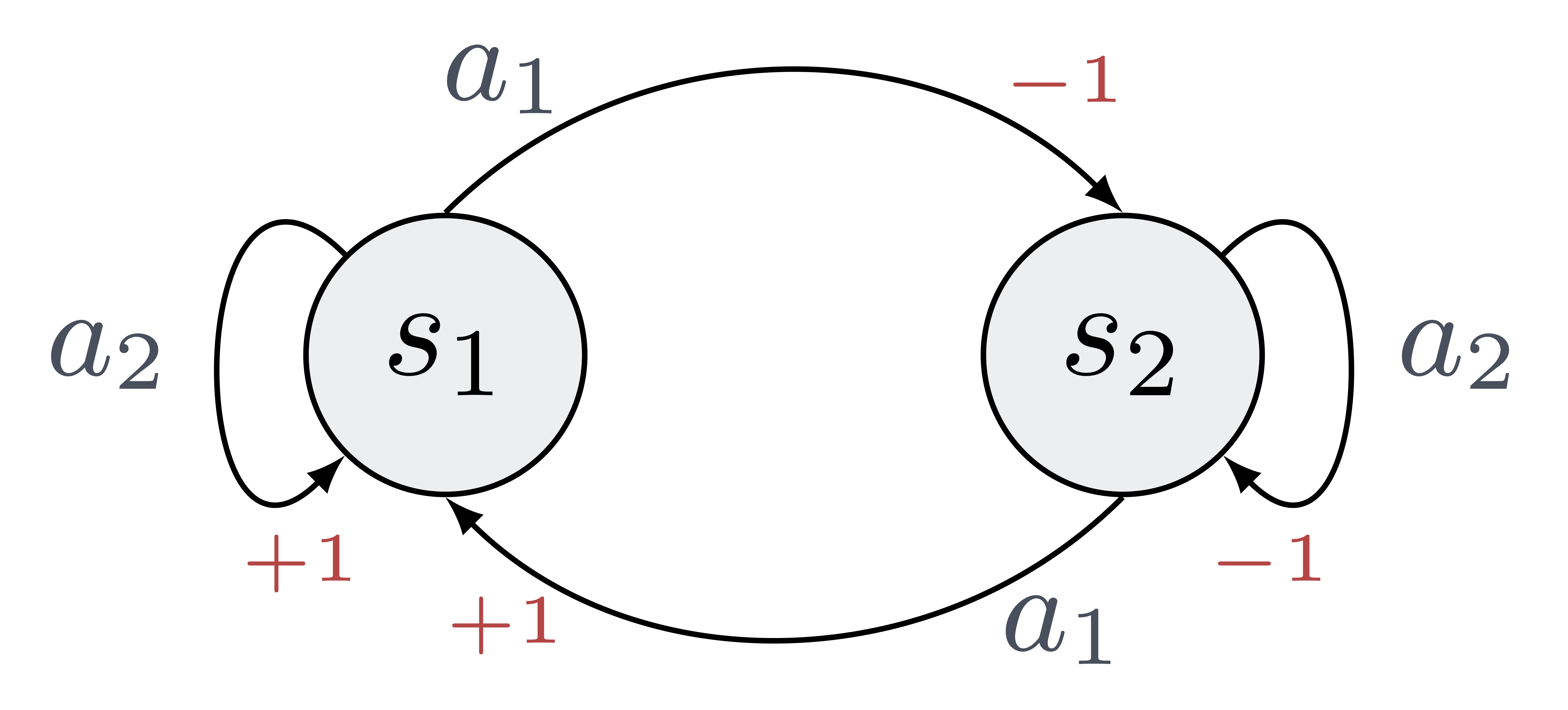
Consider the non-stationary policy $\pi = (d_1, \ldots, d_t, \ldots)\in\Pi^\text{MR}$ which almost always stays on the current node (pick $a_1$) and switches from one node to the other (pick $a_2$) on a logarithmic basis: $$ d_t(s) := \left\{\begin{aligned} &a_1 \text{ if } \log_2(t)\in\mathbb{N}\;,\\ &a_2 \text{ otherwise.} \end{aligned}\right. $$ One can show that the $T$-step average value of $\pi$ oscillates between 1/3 and -1/3; i.e $\rho_\pi$ does not exist!

▶ Proof

This sounds like bad news. However, one can easily convince oneself that in this example, all stationary policies are well-behaved and do admit an average reward $\rho_\pi$. Below, we will show that this is a general property: in finite MDPs, $\rho_\pi$ exists for any stationary policy. From now on, we will focus only on stationary policies. This is not only to ease matter; as often, we will see later down the road that for many relevant MDPs, optimal policies are indeed stationary (more precisely: we can find a stationary optimal policy).

▶ Note: infinite MDPs

Notations

$\quad$ Below, we will make heavy use of MDP vector notations.

ⓘ

In an effort to be self-contained, let’s recall some notations adopted in earlier posts that will prove useful here. We will use throughout the notation $\mathbf{P}_\pi$, referring to the transition matrix induced by $\pi$. $$ \forall s, s^\prime\in\mathcal{S}, \,\left[\mathbf{P}_\pi\right]_{ss^\prime} = p_\pi(s^\prime\vert s) := \sum_{a\in\mathcal{A}} \pi(a\vert s)p(s^\prime\vert s, a)\;. $$ Similarly, the notation $\mathbf{r}_\pi$ will denote the vector of expected rewards under $\pi$. In other words, for any $s\in\mathcal{S}$: $ \,\left[\mathbf{r}_\pi\right]_s = \sum_{a\in\mathcal{A}} \pi(a\vert s)(s, a)\; . $ We have already used those tools when studying the discounted objective. By following a similar rationale, it is straightforward to write the $T$-step value as, $$ \mathbf{v}_\pi^T = \sum_{t=1}^T \mathbf{P}_\pi^{t-1} r_\pi\; , $$ where $[\mathbf{v}_\pi^T]_s = v_\pi^T(s)$. Finally, we will denote $\boldsymbol{\rho}_\pi$ the vector notations for the average-reward value $\rho_\pi$.

Existence

The general case

We claimed earlier that in discrete MDPs, stationary policies all admit an average value. This section will rigorously prove this claim. First, observe that one can write: $$ \tag{2} \mathbf{v}_T/T = \Big(\frac{1}{T}\sum_{t=1}^T \mathbf{P}_\pi^{t-1}\Big) r_\pi\;. $$ It appears that studying the limiting behaviour of $\frac{1}{T}\sum_{t=1}^T \mathbf{P}_\pi^{t-1}$ is key to establishing the existence (or not) of a limit for $\{\mathbf{v}_T/T\}_T$, and as result of $\rho_\pi$. We will denote $\mathbf{P}_\pi^\infty$ the limiting matrix, when it exists. $$ \mathbf{P}_\pi^\infty := \lim_{T\to\infty}\frac{1}{T}\sum_{t=1}^T \mathbf{P}_\pi^{t-1}\;. $$

$\quad$ Some Markov chains reminders can prove useful here.

ⓘ

$\mathbf{P}_\pi$ is not more than the transition matrix of the Markov chain induced by $\pi$ and the transition kernel $p(\cdot)$ over $\mathcal{S}$. Would such a Markov chain be ergodic, convergence of (2) would be immediate as $\{\mathbf{P}_\pi^{t}\}_t$ would converge (this implies the convergence of the Cesaro limit). This is, however, not a necessary condition, as (2) can converge even for periodic chains. The main behaviour that (2) is fighting is periodicity–the average over time washes out any period in the stochastic process, irrelevant for computing the average reward. A typical example is $\mathbf{P}_\pi=\begin{pmatrix} 0 & 1 \\ 1 & 0\end{pmatrix}$: indeed, $\mathbf{P}_\pi^t$ does not converge but $\mathbf{P}_\pi^\infty$ does exist!

$\qquad \qquad\qquad\qquad \text{ For any stationary } \pi \text{, the matrix }\mathbf{P}_\pi^\infty\text{ exists and is right-stochastic.}$

Existence of $\mathbf{P}_\pi^\infty$

▶ Proof

A direct consequence is that in finite MDPs, $\rho_\pi$ is well defined for any stationary policy, via: $$ \tag{3} \boldsymbol{\rho}_\pi = \mathbf{P}_\pi^\infty \mathbf{r}_\pi\;. $$

Properties

The steady-state matrix $\mathbf{P}_\pi^\infty$ checks the following identity: $ \mathbf{P}_\pi\mathbf{P}_\pi^\infty = \mathbf{P}_\pi^\infty = \mathbf{P}_\pi^\infty\mathbf{P}_\pi\; $ and by (3), a similar result holds for the average reward; that is, $\mathbf{P}_\pi^\infty\rho_\pi = \rho_\pi$.

▶ Proof

We have already discussed the usefulness of $\mathbf{P}_\pi^\infty$ being a Cesaro limit of $\{ \mathbf{P}_\pi^{t}\}_t$ when the underlying chain is periodic. When said chain is aperiodic, we can simplify the definition further and write $ \mathbf{P}_\pi^\infty = \lim_{T\to\infty} \mathbf{P}_\pi^{T}\; . $

Ergodic chains

When the chain $\mathbf{P}_\pi$ is ergodic (single irreducible class and aperiodic), we know that it converges from any state to a single stationary distribution. Let $\mathbf{p}_\pi^\infty$ be this distribution. The steady-state matrix then writes $ \mathbf{P}_\pi^\infty = \begin{pmatrix} \mathbf{p}_\pi^\infty \ldots \mathbf{p}_\pi^\infty\end{pmatrix}^\top\;, $ and the average-reward: $$ \boldsymbol{\rho}_\pi = \begin{pmatrix} (\mathbf{p}_\pi^\infty)^\top\mathbf{r}_\pi \ldots (\mathbf{p}_\pi^\infty)^\top\mathbf{r}_\pi \end{pmatrix}^\top\;. $$ In other words, $\boldsymbol{\rho}_\pi$ is a constant vector; the average-reward is the same whatever the state we start from: that is, $\rho_\pi(s) = \rho_\pi(s^\prime)$ for any $s, s^\prime\in\mathcal{S}$. This is quite natural; since the contribution of the transitory regime fades away in the average reward, what remains is the steady state behaviour–which is the same whatever the starting state, and is captured by the stationary distribution. Observe that this characteristic is preserved in the presence of transient states.

The differential value function

Definition

A central quantity when studying the average reward setting is the differential value function $h_\pi$, sometimes also refered to as bias. For any $s\in\mathcal{S}$: $$ \tag{4} h_\pi(s) := \lim_{T\to\infty}\mathbb{E}_s^\pi\Big[\sum_{t=1}^T r(s_t, a_t) - \rho_\pi(s_t)\Big]\;. $$ The differential value function captures the asymptotic deviation (measured via the reward) that occurs when starting from some $s\in\mathcal{S}$ instead of the stationary distribution. Perhaps the clearest evidence of this claim arises when $\mathbf{P}_\pi$ is ergodic; $\rho_\pi$ is then state-independent, and we can write: $ h_\pi(s) := \lim_{T\to\infty}\mathbb{E}_s^\pi\Big[\sum_{t=1}^T r(s_t, a_t)\Big] - T\rho_\pi\;. $ In the more general case, another identity (left without proof) also testifies of the relationship between the differential value function and the transitory regime: $$ v_\pi^T(s) = T\rho_\pi(s) + h_\pi(s) + o_{T\to\infty}(1)\;. $$ As $T\to\infty$, the expected $T$-step value is given by a main term involving the average-reward $\rho_\pi$ and a small deviation given by the bias, capturing the fact that we did not start from the stationary distribution.

Existence

Let us write $\mathbf{h}_\pi$ the differential value function’s vectorial alter-ego. It writes $$ \mathbf{h}_\pi := \lim_{T\to\infty}\sum_{t\leq T} \mathbf{P}_\pi^t (\mathbf{r}_\pi-\boldsymbol{\rho}_\pi)\;. $$ As before, we need to prove that this limit exists. To gain some intuition as to why it does, observe that $ \mathbf{h}_\pi = \sum_{t\leq T} \big(\mathbf{P}_\pi^t-\mathbf{P}_\pi^\infty) \mathbf{r}_\pi\;. $ Intuitively, we can hope that the typical geometric convergence rate of $\mathbf{P}_\pi^t$ towards $\mathbf{P}_\pi^\infty$ will catch up to make this a convergent geometric series. That’s sadly where the intuition will stop; the existence proof we give below is rather technical, and relies on some linear algebra magic.

$\quad$ There exist more elegant and intuitive proofs to demonstrate the bias's existence. They take a probabilistic approach (tower-rule, Azuma-Hoeffding, etc.) but require tools we did not introduce here.

ⓘ

$\qquad \qquad\qquad\qquad \text{ For any stationary } \pi \text{ the differential value function } \mathbf{h}_\pi \text{ exists and is given by }:$ $$ \mathbf{h}_\pi = (\mathbf{I} - \mathbf{P}_\pi + \mathbf{P}_\pi^\infty)^{-1}(\mathbf{I}-\mathbf{P}_\pi^\infty)\mathbf{r}_\pi\;. $$

Existence of $\mathbf{h}_\pi^\infty$

▶ Proof

We will start by proving that $(\mathbf{I} - \mathbf{P}_\pi + \mathbf{P}_\pi^\infty)$ is non-singular. While proving the existence of $\mathbf{P}_\pi$ we showed that: $$ \begin{aligned} \mathbf{P}_\pi &= \mathbf{W}\begin{pmatrix} \mathbf{I}_k & 0 \\ 0 & \mathbf{Q}\end{pmatrix}\mathbf{W}^{-1}\;,\\ \mathbf{P}_\pi^\infty &= \mathbf{W}\begin{pmatrix} \mathbf{I}_k & 0 \\ 0 & 0\end{pmatrix}\mathbf{W}^{-1}\;, \end{aligned} $$ where $1\notin\text{sp}(\mathbf{Q})$ and $\sigma(\mathbf{Q})\leq 1$. As a result: $$ \mathbf{I} - \mathbf{P}_\pi + \mathbf{P}_\pi^\infty = \mathbf{W}\begin{pmatrix} \mathbf{I}_k & 0 \\ 0 & \mathbf{I}-\mathbf{Q}\end{pmatrix}\mathbf{W}^{-1} $$ where $0\notin\text{sp}(\mathbf{I}-\mathbf{Q})$, proving that $\mathbf{I} - \mathbf{P}_\pi + \mathbf{P}_\pi^\infty$ is non-singular. Now, observe that: $$ \begin{aligned} (\mathbf{I} - \mathbf{P}_\pi + \mathbf{P}_\pi^\infty )^{-1} &= \sum_{t\geq 0} (\mathbf{P}_\pi-\mathbf{P}_\pi^\infty)^{t}\;,\\ &= \sum_{t\geq 0} \sum_{k=0}^{t}\begin{pmatrix} t \\ k \end{pmatrix}(-1)^{t-k}(\mathbf{P}_\pi)^k(\mathbf{P}_\pi^\infty)^{t-k}\;, &(\text{binomial theorem})\\ &= \sum_{t\geq 0} \Big(\mathbf{P}_\pi^t + \sum_{k=0}^{t-1}\begin{pmatrix} t \\ k \end{pmatrix}(-1)^{t-k}(\mathbf{P}_\pi)^k\mathbf{P}_\pi^\infty\Big)\;, &((\mathbf{P}_\pi^\infty)^{t-k} = \mathbf{P}_\pi^\infty)\\ &= \sum_{t\geq 0} \Big(\mathbf{P}_\pi^t + \mathbf{P}_\pi^\infty\sum_{k=0}^{t-1}\begin{pmatrix} t \\ k \end{pmatrix}(-1)^{t-k}\Big)\;, &(\mathbf{P}_\pi^\infty(\mathbf{P}_\pi)^{t-k} = \mathbf{P}_\pi^\infty)\\ &= \sum_{t\geq 0} (\mathbf{P}_\pi^t - \mathbf{P}_\pi^\infty)\;. \end{aligned} $$ Further, one writes: $$ \begin{aligned} (\mathbf{I} - \mathbf{P}_\pi + \mathbf{P}_\pi^\infty )^{-1}(\mathbf{I}-\mathbf{P}_\pi)\mathbf{r}_\pi &= \sum_{t\geq 0} (\mathbf{P}_\pi^t - \mathbf{P}_\pi^\infty)\mathbf{r}_\pi\;,\\ &= \sum_{t\geq 0} \mathbf{P}_\pi^t\mathbf{r}_\pi - \mathbf{P}_\pi^t\mathbf{P}_\pi^\infty\mathbf{r}_\pi\;, &(\mathbf{P}_\pi^t\mathbf{P}_\pi^\infty=\mathbf{P}_\pi^\infty)\\ &= \sum_{t\geq 0} \mathbf{P}_\pi^t\mathbf{r}_\pi - \mathbf{P}_\pi^t\boldsymbol{\rho}_\pi\;, &(\text{def. of } \boldsymbol{\rho}_\pi)\\ &= \sum_{t\geq 0} \mathbf{P}_\pi^t\mathbf{r}_\pi - \mathbf{P}_\pi^t\boldsymbol{\rho}_\pi\;,\\ &= \sum_{t\geq 0} \mathbf{P}_\pi^t(\mathbf{r}_\pi - \boldsymbol{\rho}_\pi)\;,\\ &= \mathbf{h}_\pi\;. \end{aligned} $$

$\blacksquare$

Bellman equations

We are finally ready to give out the Bellman policy evaluation equations that characterize the average reward $\boldsymbol{\rho}_\pi$. In a following post, we will use them as the basis to establish the Bellman equations for the optimal average reward. Those will in turn be used to establish algorithms for computing optimal policies.

As anticipated, said equations involve not only $\boldsymbol{\rho}_\pi$, but also the differential value function $\boldsymbol{h}_\pi$. Concretely, let us consider the following set of equations, where $\boldsymbol{\rho}$ and $\mathbf{h}$ are both $\vert \mathcal{S}\vert$-dimensional vectors: $$ \tag{5} \left\{ \begin{aligned} &\boldsymbol{\rho} = \mathbf{P}_\pi \boldsymbol{\rho}\;, \\ &\boldsymbol{\rho} + \mathbf{h}= \mathbf{r}_\pi + \mathbf{P}_\pi\mathbf{h}\;. \end{aligned} \right. $$

$\qquad \qquad\qquad\qquad \text{Let } \pi\text{ a stationary policy and }(\boldsymbol{\rho}, \mathbf{h}) \text{ a solution to (5). Then:}$ $$ \boldsymbol{\rho}_\pi = \boldsymbol{\rho} \text{ and } \mathbf{h}_\pi = \mathbf{h} + \mathbf{u}\;, $$ $\text{ where } \mathbf{u} \text{ is any vector in the null space of }(\mathbf{P}_\pi-\mathbf{I}). \text{ Further, if } \mathbf{h} = \mathbf{P}_\pi\mathbf{h} \text{ then } \mathbf{h}_\pi = \mathbf{h}.$

Existence of $\mathbf{P}_\pi^\infty$

Concretely, the above claims $(\boldsymbol{\rho}_\pi, \mathbf{h}_\pi)$ to be the unique solution to (5) up to some element of $\text{Ker}(\mathbf{P}_\pi-\mathbf{I})$.

▶ Proof

We will start by establishing that $(\boldsymbol{\rho}_\pi, \mathbf{h}_\pi)$ is a solution to (5). We have already proven then $\boldsymbol{\rho}_\pi = \mathbf{P}_\pi \boldsymbol{\rho}_\pi$. Observe that: $$ \begin{aligned} (\mathbf{I}-\mathbf{P}_\pi)\mathbf{h}_\pi &= (\mathbf{I}-\mathbf{P}_\pi) (\mathbf{I} - \mathbf{P}_\pi + \mathbf{P}_\pi^\infty)^{-1}(\mathbf{I}-\mathbf{P}_\pi^\infty)\mathbf{r}_\pi\;, \\ &\overset{(i)}{=} (\mathbf{I}-\mathbf{P}_\pi)\sum_{t\geq 0}(\mathbf{P}_\pi^t-\mathbf{P}_\pi^\infty)\mathbf{r}_\pi\;,\\ &= \Big(\sum_{t\geq 0}(\mathbf{P}_\pi^t-\mathbf{P}_\pi^\infty) - \sum_{t\geq 1}(\mathbf{P}_\pi^t-\mathbf{P}_\pi^\infty)\Big)\mathbf{r}_\pi\;, &(\mathbf{P}_\pi\mathbf{P}_\pi^\infty=\mathbf{P}_\pi^\infty))\\ &= (\mathbf{I}-\mathbf{P}_\pi^\infty)\mathbf{r}_\pi\;, &(\text{telescopic sum})\\ &= \mathbf{r}_\pi - \boldsymbol{\rho}_\pi\;. &(\boldsymbol{\rho}_\pi=\mathbf{P}_\pi^\infty\mathbf{r}_\pi) \end{aligned} $$ where $(i)$ was taken from an earlier proof about the existence of $\mathbf{h}_\pi$. Hence, $(\boldsymbol{\rho}_\pi, \mathbf{h}_\pi)$ is a solution to (5).

Now, let $(\boldsymbol{\rho}, \mathbf{h})$ be a solution to (5). Multiplying the second identity in (5) by $\mathbf{P}_\pi^\infty$ on the left, we obtain: $$ \begin{aligned} 0 &= \mathbf{P}_\pi^\infty\boldsymbol{\rho} - \mathbf{P}_\pi^\infty\mathbf{r}_\pi + \mathbf{P}_\pi^\infty\mathbf{h} - \mathbf{P}_\pi^\infty\mathbf{P}_\pi\mathbf{h} \;, \\ &= \boldsymbol{\rho} - \mathbf{P}_\pi^\infty\mathbf{r}_\pi + \mathbf{P}_\pi^\infty\mathbf{h} - \mathbf{P}_\pi^\infty\mathbf{P}_\pi\mathbf{h} \;, & (\text{by (5)})\\ &= \boldsymbol{\rho} - \boldsymbol{\rho}_\pi + \mathbf{P}_\pi^\infty\mathbf{h} - \mathbf{P}_\pi^\infty\mathbf{P}_\pi\mathbf{h} \;, &(\text{def of }\boldsymbol{\rho}_\pi)\\ &= \boldsymbol{\rho} - \boldsymbol{\rho}_\pi + \mathbf{P}_\pi^\infty\mathbf{h} - \mathbf{P}_\pi^\infty\mathbf{h} \;, &(\mathbf{P}_\pi^\infty\mathbf{P}_\pi=\mathbf{P}_\pi^\infty)\\ &= \boldsymbol{\rho} - \boldsymbol{\rho}_\pi\;, \end{aligned} $$ establishing that $\boldsymbol{\rho} = \boldsymbol{\rho}_\pi$. Substracting together the second identity of (5) taken, respectively, in $(\boldsymbol{\rho}, \mathbf{h})$ and $(\boldsymbol{\rho}_\pi, \mathbf{h}_\pi)$, we obtain: $$ \begin{aligned} 0 &= \boldsymbol{\rho} - \boldsymbol{\rho}_\pi + \mathbf{h} - \mathbf{h}_\pi - \mathbf{P}_\pi(\mathbf{h}-\mathbf{h}_\pi)\;,\\ 0 &=\mathbf{h} - \mathbf{h}_\pi - \mathbf{P}_\pi(\mathbf{h}-\mathbf{h}_\pi)\;, &(\boldsymbol{\rho} = \boldsymbol{\rho}_\pi) \end{aligned} $$ or in other words that $(\mathbf{I}-\mathbf{P}_\pi)(\mathbf{h}-\mathbf{h}_\pi)=0$, which finishes to establish our claim as $(\mathbf{h}-\mathbf{h}_\pi)\in\text{Ker}(\mathbf{I}-\mathbf{P}_\pi)$.

$\blacksquare$

When the chain $\mathbf{P}_\pi$ is ergodic, we saw that $\boldsymbol{\rho}_\pi$ is a constant vector; we write $\boldsymbol{\rho}_\pi = {\rho}_\pi \mathbf{1}$ where $\mathbf{1}$ is an $\vert\mathcal{S}\vert$-dimensional vector, where all entries are 1. In this context, the identity $\boldsymbol{\rho}_\pi = \mathbf{P}_\pi \boldsymbol{\rho}_\pi$ is redundant since $\mathbf{P}_\pi\mathbf{1}=\mathbf{1}$ – it would basically boil down to ${\rho}_\pi={\rho}_\pi$ which is not the most useful thing to learn about ${\rho}_\pi$! In this case, the Bellman policy evaluation equation for the average-reward is reduced to a single identity: $$ \tag{6} \rho_\pi\mathbf{1} + \mathbf{h}_\pi= \mathbf{r}_\pi + \mathbf{P}_\pi\mathbf{h}\;. $$ In a following post, we will introduce some (non-degenerate) MDP classes for which the optimal policy is ergodic, and therefore satisfies (6). This identity will therefore serve as our springboard to establish the Bellman equations for optimality under the average reward criterion.

References

This blog-post is a condensed and simplified version of [Puterman. 94, Chapter 8]. For digging even further, [Arapostathis et. al. 93] is an amazing resource.