MDP Fundamentals (2/3)

In this second blog post of the series, we cover the problem of value prediction and control in finite discounted MDPs. This will lead us in particular to review the Bellman prediction and control equations, and to a fundamental theorem of MDPs: stationary policies are enough for optimal control!

$\;\;\;$ Before diving in, make sure you've read the previous blog-post on MDPs. Recall that we use vectorial notations, and adopt the usual partial ordering over $\mathbb{R}^n$: $$ x \geq y \Longleftrightarrow x_i \geq y_i \; \text{ for all } i\in\{1,\ldots, n\} \; . $$

ⓘ

Our ultimate goal here is to derive some characterisation of an optimal policy for a discounted MDP. Said optimal policy would check: $$ \pi^\star \in \argmax_{\pi \in \Pi^\text{HR}} v_\lambda^\pi(s) \text{ for all } s \in\mathcal{S} . $$ We will use the shorthand $v_\lambda^\star:=v_\lambda^{\pi^\star}$ to denote the optimal value function, which therefore checks: $$ v_\lambda^\star = \max_{\pi \in \Pi^\text{HR}} v_\lambda^\pi\; . $$

Warm-up: Policy Evaluation

This first part is concerned with policy evaluation: given some stationary policy $\pi\in\mathcal{S}^\text{MD}$, what recurrence property its discounted value $v_\lambda^\pi$ satisfies? This question can at first seem like a side-quest on our path (after all, we are mostly concerned with optimal policies, not just any policy). It will however serve as a gentle introduction for the rest of the blog-post.

Let’s dive in with the first technical result, which establishes the Bellman prediction equations. Let $\pi=(d, d, \ldots)\in\mathcal{S}^\text{MD}$ a stationary policy. Then, its expected discounted value $v_\lambda^\pi$ is the unique bounded function from $\mathcal{S}$ to $\mathbb{R}$ which satisfies for all $s\in\mathcal{S}$;

$$ v_\lambda^\pi(s) = r(s, d(s)) + \lambda\mathbb{E}\big[v_\lambda^\pi(s’)\big] \text{ where } s’\sim p(\cdot\vert s, d(s))\; . $$

In our discrete setting we can naturally rewrite this using sums: $$ \begin{aligned} \; v_\lambda^\pi(s) &= r(s, d(s)) + \lambda\sum_{s’\in\mathcal{S}} v_\lambda^\pi(s’)\mathbb{P}\left(s_{t=1}=s’\middle\vert s_t=s, a_t=d(s)\right)\; , \end{aligned} $$ and finally have the very compact vector notation when $\mathcal{S}$ is finite: $$ v_\lambda^\pi = \mathbf{r}_{d} + \lambda \mathbf{P}_{d}v_\lambda^\pi\; . $$

▶ Proof

In the finite case the above proof yields a neat characterisation of the discounted expected cost of a stationary policy: $$ v_\lambda^\pi = (\mathbf{I}_n - \lambda\mathbf{P}_{d}) ^{-1}\mathbf{r}_{d}\; . $$

There is yet one last way of writing the Bellman prediction equation which will prove useful. For any policy $\pi=(d, \ldots) \in\mathcal{S}^\text{MR}$, let us introduce the policy evaluation operator $\mathcal{T}_\lambda^\pi$:

$$ \begin{aligned} \mathcal{T}_\lambda^d : \mathcal{V}&\mapsto \mathcal{V} \\ f &\mapsto \mathcal{T}_\lambda^d(f) \; \text{ where } \; \mathcal{T}_\lambda^d(f)(s):= r(s, d(s)) + \lambda\mathbb{E}^{d}_s\big[f(s_{t+1})\big] \; . \end{aligned} $$

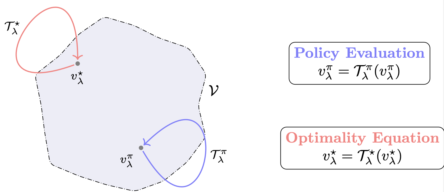
We can therefore neatly write that the discounted expected value of some policy is the unique fixed-point of its associated policy evaluation operator:

$$ { v_\lambda^\pi = \mathcal{T}_\lambda^d(v_\lambda^\pi) \; . } $$

Bellman prediction equations

Optimal Control

We can now move on to the characterisation of the optimal expected discounted cost $v_\lambda^\star$. The Bellman optimality equations for the discounted case draw their intuition from the finite horizon case. Since we haven’t covered it explicitly, we will simply claim their discounted counterpart and proceed with proving that they indeed characterise optimal policies.

Formally, we say that $f\in\mathcal{V}$ satisfies the Bellman optimality equations for discounted MDPs if:

$$ \begin{aligned} \forall s\in\mathcal{S}, \; f(s) = \max_{a\in\mathcal{A}} \left\{ r(s,a) + \lambda\mathbb{E}\left[f(s_{t+1})\middle\vert s_t=s, a_t=a\right] \right\}\; . \end{aligned} $$

We can also write the above identity as: $ f = \mathcal{T}_\lambda^\star(f) $, where we defined the Bellman optimality operator: $$ \begin{aligned} \mathcal{T}_\lambda^\star : \mathcal{V}&\mapsto \mathcal{V} \\ f &\mapsto \mathcal{T}_\lambda^\star(f) := \max_{d\in\mathcal{D}^\text{MD}} \mathcal{T}_\lambda^d(f)\; . \end{aligned} $$

It turns out that if $f\in\mathcal{V}$ satisfies this identity, then $f=v_\lambda^\star$! In others word, the optimal expected discounted cost is the unique solution to Bellman’s optimality equations - or equivalently the unique fixed point of the operator $\mathcal{T}_\lambda^\star$.

▶ Proof

Let $f\in\mathcal{V}$ such that for all $s\in\mathcal{S}$. The proof goes by establishing the following claims:

$f \leq \mathcal{T}_\lambda^\star(f)$ then $f \leq v_\lambda^\star$,
$f \geq \mathcal{T}_\lambda^\star(f)$ then $f \geq v_\lambda^\star$,
$f = \mathcal{T}_\lambda^\star(f)$ then $f = v_\lambda^\star$,

where we again adopt the classical partial ordering over vectors. Let’s first prove the first claim. Let $f(s) \geq \mathcal{T}_\lambda^\star(f)$ for all $s\in\mathcal{S}$. Then for any $d\in\mathcal{D}^\text{MD}$: $$ \begin{aligned} f &\leq \mathbf{r}_{d} + \lambda\mathbf{P}_{d}f\; , \\ \Longleftrightarrow &(\mathbf{I}_n-\lambda\mathbf{P}_{d})f \leq \mathbf{r}_{d}\; . \end{aligned} $$ Using the fact that $(\mathbf{I}_n-\lambda\mathbf{P}_{d})^{-1} = \sum_{k=0}^\infty \lambda^k\mathbf{P}_{d}^k $ which only has positive entries, we obtain that; $$ \begin{aligned} f &\leq (\mathbf{I}_n-\lambda\mathbf{P}_{d})^{-1}( \mathbf{r}_{d})\\ &= v_\lambda^{\pi} \; , \end{aligned} $$ for any $\pi = (d, \ldots) \in\mathcal{S}^\text{MD}$ (we just used the characterisation of a stationary policy). Therefore: $$f \leq \max_{\pi\in\mathcal{S}^\text{MR}} v_\lambda^\pi\leq \max_{\pi\in\Pi^\text{HR}} v_\lambda^\pi= v_\lambda^\star\; . $$

We now prove the second claim. Observe that if $f \leq \mathcal{T}_\lambda^\star(f)$ then for any $d_1, d_2, \ldots \in\mathcal{D}^\text{MR}$: $$ \begin{aligned} f &\leq \mathbf{r}_{d_1} + \lambda\mathbf{P}_{d_1} f \; \\ &\leq \mathbf{r}_{d_1} + \lambda\mathbf{P}_{d_1}\mathbf{r}_{d_2} + \lambda^2 \mathbf{P}_{d_2} f\;, \\ &\leq \ldots \\ &\leq \sum_{t=1}^\tau \lambda^{t-1}\mathbf{P}_{\pi}^t\mathbf{r}_{d_t} + \lambda^\tau \mathbf{P}_{\pi}^\tau\mathbf{r}_{d_\tau}\; . \end{aligned} $$ Since $\lambda < 1$ and $\mathbf{P}_{\pi}^\tau$ is stochastic, we have $\lim_{\tau\to\infty}\lambda^\tau \mathbf{P}_{\pi}^\tau\mathbf{r}_{d_\tau} = 0$ and therefore: $$ f \leq \sum_{t=1}^\infty \lambda^{t-1}\mathbf{P}_{\pi}^t\mathbf{r}_{d_t} = v_\lambda^\pi\; , $$ for any $\pi = (d_1, d_2 \ldots, ) \in\Pi^\text{MR}$. Hence $f\leq \max_{\pi\in\Pi^\text{MR}}v_\lambda^\pi = \max_{\pi\in\Pi^\text{HR}}v_\lambda^\pi$. The third claim is easily obtained by combining the first two.

We are now left with proving that such a solution exists – equivalently, that $\mathcal{T}_\lambda^\star$ indeed admits a fixed point. The technical tool to achieve this is the Banach’s fixed point theorem. The key claim of this theorem is that if some operator acting on a space without holes (a.k.a complete) is contracting, then it must admit a unique fixed point. Turns out, the Bellman optimality operator is contracting. Indeed, for all $f, g\in\mathcal{V}$: $$ \left\lVert \mathcal{T}_\lambda^\star(f) - \mathcal{T}_\lambda^\star(g) \right\rVert_\infty \leq \lambda \left\lVert f - g\right\rVert_\infty < \left\lVert f - g\right\rVert_\infty\; . $$

▶ Proof

Observe that for any $d\in\mathcal{D}^\text{MD}$ the operator $\mathcal{T}_\lambda^\pi$ is itself contracting, since for all $f,g\in\mathcal{V}$: $$ \begin{aligned} \| \mathcal{T}_\lambda^d(f) - \mathcal{T}_\lambda^d(g)\|_\infty &= \| \lambda \mathbf{P}_{d}(f-g)\|_\infty\; , \\ &\leq \lambda \| \mathbf{P}_{d}\|_\infty\|f-g\|_\infty\ ,&(\text{operator norm property})\\ &\leq \lambda\|f-g\|_\infty\; . & (\mathbf{P}_{d} \text{ stochastic}) \end{aligned} $$ The fact that $\mathcal{T}_\lambda^\star = \inf{d\in\mathcal{D}^\text{MD}} \mathcal{T}_\lambda^d$ finishes the proof; indeed for all $f, g\in\mathcal{V}$ let $d_f = \argmax \mathcal{T}_\lambda^d f$. Then: $$ \begin{aligned} \mathcal{T}_\lambda^\star(f) - \mathcal{T}_\lambda^\star(g) &= \mathcal{T}_\lambda^{d_f}(f) - \mathcal{T}_\lambda^\star(g)\\ &\leq \mathcal{T}_\lambda^{d_f}(f) -\mathcal{T}_\lambda^{d_f}(g)\; . \end{aligned} $$ This mean that for any $s\in\mathcal{S}$ we have $$\mathcal{T}_\lambda^\star(f)(s) - \mathcal{T}_\lambda^\star(g)(s) \leq \mathcal{T}_\lambda^{d_f}(f)(s) -\mathcal{T}_\lambda^{d_f}(g)(s)$$. Assuming for now that $\mathcal{T}_\lambda^\star(f)(s) - \mathcal{T}_\lambda^\star(g)(s)\geq 0$ yields that: $$ \begin{aligned} 0 \leq \mathcal{T}_\lambda^\star(f)(s) - \mathcal{T}_\lambda^\star(g)(s)\leq \mathcal{T}_\lambda^{d_f}(f)(s) -\mathcal{T}_\lambda^{d_f}(g)(s) \;,\\ \end{aligned} $$ Therefore: $$ \begin{aligned} \mathcal{T}_\lambda^{d_f}(f)(s) -\mathcal{T}_\lambda^{d_f}(g)(s) &\leq \vert \mathcal{T}_\lambda^{d_f}(f)(s) -\mathcal{T}_\lambda^{d_f}(g)(s)\vert \; , \\ &\leq \lVert \mathcal{T}_\lambda^{d_f}(f) -\mathcal{T}_\lambda^{d_f}(g)\rVert \; ,\\ &\le \lambda \| f -g \| \; . \end{aligned} $$ This yields the desired result when $ \mathcal{T}_\lambda^\star(f)(s) \geq \mathcal{T}_\lambda^\star(g)(s)$. The completementy case is easily dealt by a reverse argument – studying $ \mathcal{T}_\lambda^\star(g) - \mathcal{T}_\lambda^\star(f)$ instead of $ \mathcal{T}_\lambda^\star(f) - \mathcal{T}_\lambda^\star(g)$.

This completes this section. We have proven that $\mathcal{T}_\lambda^\star$ admits a unique fixed point, which is the optimal value function. The optimal value function $v_\lambda^\star$ is therefore the only function which satisfies the Bellman’s optimality equations.

$$ { v_\lambda^\star = \mathcal{T}_\lambda^\star(v_\lambda^\star) = \max_{d\in\mathcal{D}^\text{MD}} \mathcal{T}_\lambda^d (v_\lambda^\star)\; . } $$

Bellman control equations

Optimal Policies

When it comes to optimality, we have so far focused on history-dependent randomised policies, then on Markov randomised policies. From a computational standpoint, it would be desirable to be able to restrict this policy space even further–and focus only on stationary policies. Indeed, a stationary policy is made up of a single decision-rule and is therefore easy to store and update. For this restriction to be principled, we are missing one fundamental result which ensures that the optimal discounted cost is attained by a stationary policy. We will need the notion of a conserving decision-rule; we say that $d^\star\in\mathcal{D}^\text{MD}$ is conserving or $v_\lambda^\star$-improving if for all $s\in\mathcal{S}$;

$$ \begin{aligned} r(s,d^\star(s)) + \mathbb{E}\left[v_\lambda^\star(s_{t+1})\middle\vert s_t=s, a_t=d^\star(s)\right] := \max_{a\in\mathcal{A}}\left\{ r(s, a) + \mathbb{E}\left[v_\lambda^\star(s_{t+1})\middle\vert s_t=s, a_t=a\right]\right\}\; . \end{aligned} $$ Equivalently, $d^\star\in\argmax_{d\in\mathcal{D}^\text{MD}} \mathbf{r}_d + \lambda\mathbf{P}_d v_\lambda^\star$. Then the stationary policy $\pi^\star = (d^\star, \ldots)$ is optimal: $$ v_\lambda^\star = \max_{\pi\in\Pi^\text{HR}} v_\lambda^\pi = v_\lambda^{\pi^\star}\; . $$

▶ Proof

Behind this somewhat simple result lies what is sometimes called the fundamental theorem of MDPs, ensuring us that we can confidently turn away from history-dependent policies and focus on (Markovian) stationary ones.

$$ \max_{\pi\in\Pi^\text{HR}} v_\lambda^\pi = \max_{\pi\in\mathcal{S}^\text{MD}} v_\lambda^\pi \; . $$

Fundamental theorem of MDPs

Beyond discrete action spaces

We have focused so far on discrete MDPs – with discrete state and action spaces. Most result are portable beyond this setting, and extend to continuous action spaces. In this case, the optimal value function becomes the solution of a supremum problem (since there then exists a continuously infinite number of policies): $$ v_\lambda^\star = \sup_{\pi\in\Pi^\text{HR}} v_\lambda^\pi \; . $$ The Bellman optimality operator becomes, for any $f\in\mathcal{V}$: $$ \mathcal{T}_\lambda^\star(f) = \sup_{d\in\mathcal{D}^\text{MD}} \{ \mathbf{r}_d + \lambda\mathbf{P}_d \cdot f \} \; . $$ Whenever this supremum is reached (i.e. when the reward and transition function are continuous – or even only upper semi-continuous – and the action space compact) then one can show that again, there exists an optimal stationary policy.

Resources

Most of this blog-post is a condensed version of [Puterman. 94, Chapter 4&5] See the previous blog post on MDPs here.