This blog-post is concerned with computational methods for finding optimal policies. We will cover Value Iteration (VI) and Policy Iteration (PI), which serve as fundamental building blocks for many modern RL methods. We will also quickly cover the Generalized Policy Iteration approach, on top of which stand all fancy modern actor-critic methods.

Reminders

Recall that the optimal discounted cost function $v_\lambda^\star$ is the unique fixed point of $\mathcal{T}_\lambda^\star$; $$ v_\lambda^\star = \mathcal{T}_\lambda^\star(v_\lambda^\star) \;\text{ where }\; \mathcal{T}_\lambda^\star(f) =\max_{d\in\mathcal{D}^\text{MD}} \{ \mathbf{r}_{d} + \lambda\mathbf{P}_{d}\cdot f\} \; . $$ Also keep in mind that an optimal policy can be computed by finding a conserving decision-rule $d^\star$: $$ d^\star \in \argmax_{d\in\mathcal{D}^\text{MD}} \{\mathbf{r}_{d} + \lambda\mathbf{P}_{d}\cdot v_\lambda^\star\} \; . $$ and forming the stationary policy $\pi^\star = (d^\star , d^\star, \ldots)$.

Value Iteration

The Value Iteration (VI) is a value-based method. It works by first trying to compute $v_\lambda^\star$ in a recursive fashion. Once a decent approximation is computed, and only then, a near optimal policy will be computed.

Algorithm

A fundamental property of the optimal value function lies in the fact that it is the unique fixed-point of the contracting mapping $\mathcal{T}_\lambda^\star$. We can use that to our advantage, as it means that applying $\mathcal{T}_\lambda^\star$ to any vector $f\in\mathcal{V}$ gets us a bit closer to $v_\lambda^\star$. Actually, we just described the main rationale behind Value Iteration!

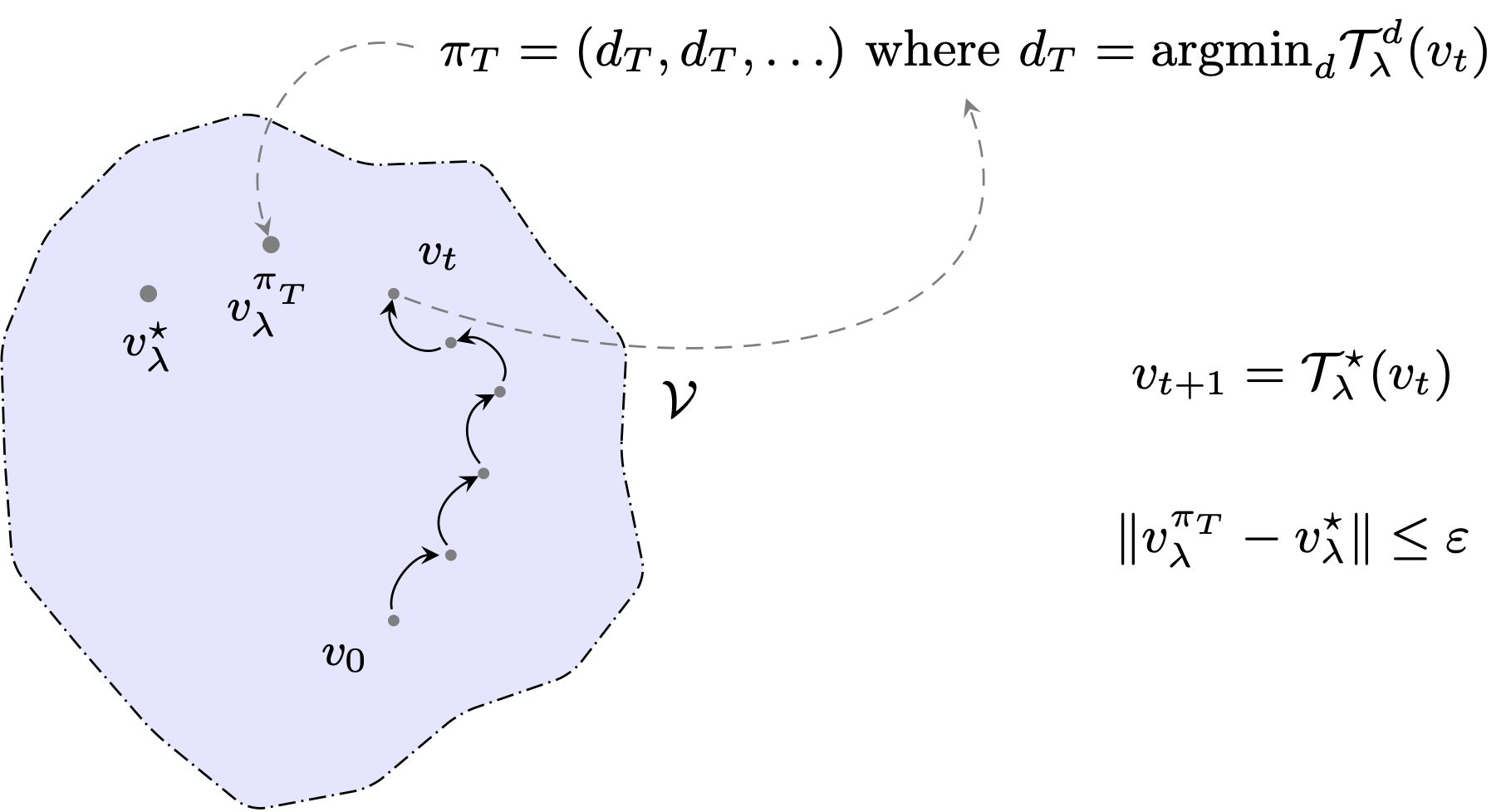
Indeed, Value Iteration works by repeatedly applying $\mathcal{T}_\lambda^\star$ to an initial guess $v_0\in\mathcal{V}$. That’s it! After a while, we will obtain some estimate $v_t$ of $v_\lambda^\star$. We can extract a $v_t$-improving decision-rule: $$ d_t \in \argmax_{d\in\mathcal{D}^\text{MD}} \left\{ \mathbf{r}_d + \lambda\mathbf{P}_d \cdot v_t\right\} \; , $$ and form the policy $\pi_t = (d_t, d_t, \ldots)\in\mathcal{S}^\text{MD}$ – hoping that it will not be too far from $\pi^\star$! Actually, we can do better than hope: we’ll shortly see that by having $t$ large enough we can arbitrarily control the sub-optimality gap suffered by $\pi_t$. Let’s first recap the Value Iteration algorithm, this time without vectorial notations for clarity:

We can also decide to write in a more compact way: $$ \begin{aligned} v_{t+1} &= \mathcal{T}_\lambda^\star (v_{t}),\; \qquad\forall t=0,\ldots, T-1 \; , \\ d_T &= \argmax_{d\in\mathcal{D}^\text{MD}} \mathcal{T}_\lambda^d(v_{T}) \; . \end{aligned} $$

Convergence properties

The first important property of the VI algorithm is that its value estimate $\{ v_t \}_t$ converge to the optimal value function: $$ v_t \overset{t\to\infty}{\longrightarrow} v_\lambda^\star\; . $$ That’s actually a by-product of Banach’s fixed-point theorem, which was used to prove the very existence of $v_\lambda^\star$! In that sense, you can consider that VI is nothing more than a glorified fixed-point algorithm.

If $T$ is large enough, then $v_T$ will be relatively close to $v_\lambda^\star$, and the $v_T$-improving policy should be a decent one. This is formalised below, where we establish that we can actually make VI output policies that are arbitrarily close to being optimal. The symbol ${\small\blacksquare}$ denotes numerical constants, removed to reduce clutter.

Policy Iteration

While the VI algorithm can be thought of as an application of a general approach for discovering fixed-point, the Policy Iteration (PI) algorithm instead leverages the very structure of MDPs.

Algorithm

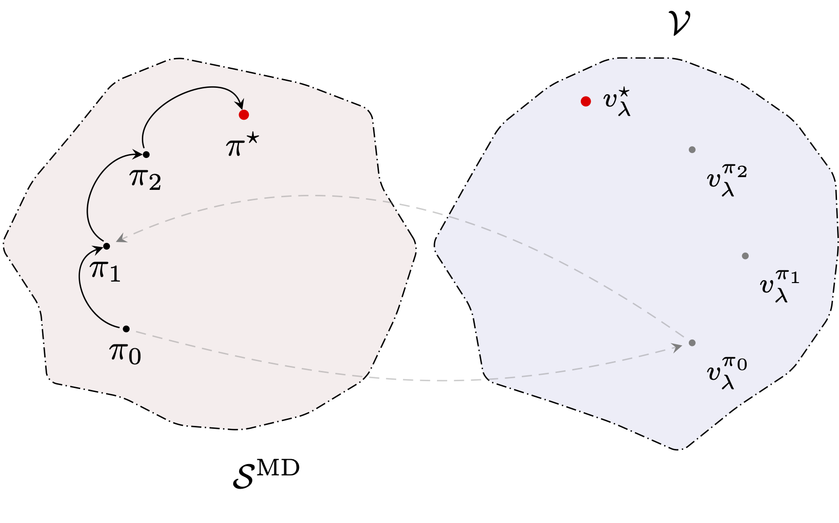
PI is a policy-based method; instead of refining approximations of the optimal discounted cost $v_\lambda^\star$, it maintains a sequence of decision-rules $\{d_t\}_t$ (or equivalently a sequence of stationary policies) approaching the optimal decision-rule $d^\star$. The main idea to achieve this is to repeatedly “improve” over the last policy; formally at round $t$ and by denoting $\pi_t=(d_t, d_t, \ldots)$, the PI algorithm defines the next iterate as: $$ d_{t+1} \in \argmax_{d\in\mathcal{D}^\text{MD}}\left\{ \mathbf{r}_{d} + \lambda\mathbf{P}_{d}\cdot v_\lambda^{\pi_t}\right\} \; . $$ The PI algorithm therefore alternates between two independent mechanisms: (1) the evaluation the current policy, meaning computing the value of the current policy $\pi_t = (d_t, d_t, \ldots)$ ad (2) the improvement of said policy by computing $d_{t+1}$ as detailed above. To match with our description of VI, we present below a version of the pseudocode where we start by policy improvement.

The policy evaluation step is left here somewhat blurry. We know that $v_\lambda^{\pi_{t+1}}$ is the unique fixed-point of $\mathcal{T}_\lambda^{d_{t+1}}$, hence the only requirement we ask is that $v_{t+1}$ is a solution of that fixed-point equation. In finite MDPs, we saw that a straight-forward solution is to write directly: $$ v_{t+1} = (\mathbf{I}-\lambda\mathbf{P}_{d_{t+1}})^{-1}\mathbf{r}_{d_{t+1}} \; . $$

Convergence properties

A core property of PI lies in its monotonic improvement. Indeed, we first make the observation that PI produces a sequences of non-decreasing discounted costs.

It turns out that in our finite setting this is enough to guarantee the convergence of PI in a finite number of iterations. Indeed, in the finite case, there exists only a finite number of decision-rules (precisely $\vert\mathcal{A}\vert^{\vert\mathcal{S}\vert}$ many ones) and the PI algorithm exhausts them in increasing order of their discounted return. Note that no loop over the policies can arise since the equality case $v_\lambda^{\pi_{t+1}} \leq J_\lambda^{\pi_{t}}$ implies that: $$ \mathcal{T}_\lambda^\star(v_\lambda^{\pi_{t}}) = v_\lambda^{\pi_{t}}\; , $$ and therefore that $v_\lambda^{\pi_{t}}=v_\lambda^\star$ – meaning that the PI algorithm will return $d^\star$ at the following iteration.

This finite-time convergence, of course, does not extend to countable MDPs, where the number of policies is (countably) infinite. It’s however fairly straightforward to also establish convergence rates for the PI algorithm; one will find out that, as VI, it enjoys linear convergence.

Generalised Policy Iteration

Computational Costs

We have so far avoided any discussion around computation cost. It’s fairly easy to establish that running each algorithm for $T$ steps roughly requires the following number of operations: $$ \begin{aligned} \text{V.I } \quad \longrightarrow \quad &\mathcal{O}(T\vert\mathcal{S}\vert^2\vert\mathcal{A}\vert) \;,\\ \text{P.I } \quad \longrightarrow \quad & \mathcal{O}(T\vert\mathcal{S}\vert^2\vert\mathcal{A}\vert + T \vert \mathcal{S} \vert^3)\;. \end{aligned} $$ As its rather common to have $\vert \mathcal{S} \vert \gg \vert \mathcal{A} \vert$ the computational cost of PI is often dominated by its policy evaluation step which requires around $\mathcal{O}(\vert \mathcal{S} \vert^3 $) operations. On the other hand, whenever $\vert \mathcal{A} \vert$ grows large, both algorithms see there efficiency drop as improving policies or value functions would require a linear scan of the action space. The problem is even tougher for continuous action spaces (e.g. $\mathcal{A} = \mathbb{R}$) since then, at each step and for each state, one has to solve a continuous, potentially non-convex optimisation problem.

Rationale

The Generalised Policy Iteration (GPI) framework allows us to overcome such computational limitations, while retaining some of the enjoyable convergence properties of VI and PI. The idea is quite simple. Instead of alternating between fully complete Policy Evaluation and Policy Improvement steps, one can decide to solve each of them only approximately before switching to the other.

For concreteness, let’s first focus on the Policy Evaluation step. In the following let $\pi$ some arbitrary stationary policy. It’s important to realise than solving the system $v_\lambda ^\pi = \mathcal{T}_\lambda^\pi(v_\lambda ^\pi)$ can be done several ways – not only by inverting some large matrix. This is a fixed-point equation for the mapping $\mathcal{T}_\lambda^\pi$, which happens to be contracting. For the very same reasons that VI’s iterates converge to $v_\lambda^\star$, the sequence: $$ v_{t+1} = \mathcal{T}_\lambda^\pi(v_t) $$ will check $v_t \overset{t\to\infty}{\longrightarrow} v_\lambda^\pi$. Such a procedure perfectly fits the GPI framework. Indeed, instead of bringing this iterative process to full convergence, we could decide to stop prematurely and pass some $v_T$ as an approximation of $v_\lambda^\pi$. If this approximation is reasonable, overall the process will still output gracefully improving policies.

Similarly, the Policy Improvement step can be degraded. Instead of finding a $v_\lambda^{\pi_t}$-improving policy, it could be enough to find $d_{t+1}$ such that for all $s\in\mathcal{S}$: $$ \begin{aligned} r(s,d_{t+1}(s)) + \lambda\sum_{s’\in\mathcal{S}} \mathbb{P}(s_{t+1}=s’\vert s_t=s, a_t=d_{t+1}(s)) v_{t}(s’)&\\ &\geq \\ &r(s,d_{t}(s)) + \lambda\sum_{s’\in\mathcal{S}} \mathbb{P}(s_{t+1}=s’\vert s_t=s, a_t=d_t(s)) v_{t}(s’) \end{aligned} $$

Example

Value Iteration

Value Iteration is actually only a special case of GPI. Indeed, if one decides to follow only 1-step of the iterative Policy Evaluation procedure we just described, we then have $$ \begin{aligned} v_{t+1} &= \mathcal{T}_\lambda^{d_{t+1}}(v_t) \;,\\ &=\mathcal{T}_\lambda^{\star}(v_t) \;, \end{aligned} $$ since by definition $d_{t+1}(s) \in \argmax_{a\in\mathcal{A}} \Big\{ r(s,a) + \lambda\sum_{s’\in\mathcal{S}} \mathbb{P}(s_{t+1}=s’\vert s_t=s, a_t=a) v_{t}(s’)\Big\}$.

Actor-Critic Algorithms

Most deep-learning based actor-critic algorithms (e.g. PPO, SAC) rely on the GPI framework. Parametric policies $\pi_\theta$ are improved via gradient-based optimisation (thanks to some policy gradient estimates) while another parametric function $v_\phi$ is trained to estimate $v_\lambda^{\pi_\theta}$ via, e.g. Bellman residual minimisation: $$ \phi \in\argmin \sum_{s} \left(v_\phi(s) - r(s, a) - \lambda v_\phi(s’)\right)^2\;, \qquad a\sim\pi_\theta(s), \;s’\sim p_t(\cdot\vert s, a)\; . $$

Others

Without jumping all the way to modern deep-learning approaches, several mechanisms have been devised to perform each step (evaluation and improvement) as quickly as possible while retaining most of the PI’s performances (e.g. Prioritised Value Iteration). The interested reader is referred to [Mausam & Kolobov, 2012] for a detailed review.

Resources

The description of VI and PI is a condensed version of [Puterman. 94, Chapter 6]