Partially Observable MDPs allow to model sensor noise, data occlusion, .. in Markov Decision Processes. Partial observability is unquestionably practically relevant, but at first glance this richer interaction setting seems to invalidate the fundamental theorem of MDPs, a.k.a the sufficiency of stationary policies. The goal of this post is to nuance this last statement: we will detail how POMDPs really are just “large” MDPs and therefore enjoy many of the same features.

PODMPs

In a Partially Observable Markov Decision Process, the actual state of the system is not available to the agent: only an observation of the state is. This observation could be, for instance, some noisy version of the state (imperfect sensor) or a partial view of it (i.e. a camera observing a robot can only report the robot’s position, not its speed). The agent must therefore base its actions only on said observations, without perfect state knowledge. Before discussing the main implications behind this stark difference with fully observed MDPs, let’s first clarify what we mean by observations. We will stay true to our MDP series and stick with finite state and actions spaces for simplicity. Similarly, the observation space will remain finite.

Observation model

The basic ingredients of MDPs are still relevant for POMDPs. From our MDP series we will keep our notations for the state space $\mathcal{S}$, the action space $\mathcal{A}$, the cost function $r$ and the state transition kernel $p$. To this mix we add a finite observation space $\Omega$ ($\vert\Omega\vert < \infty$) as well observation kernel $q(\cdot\vert s)$ which describes the conditional probability of witnessing some observation given a state. This probability mass function is sometimes referred to as the emission likelihood. Formally, for all $s, \omega \in\mathcal{S}\times\Omega$: $$ q(\omega\vert s) = \mathbb{P}\big(\omega_t = \omega \big\vert s_t = s\big)\; . $$

The decision-making process unrolls as follows; after the agent inputs $a_t$, the state transitions to $s_{t+1}\sim p(\cdot\vert s_t, a_t)$ and outputs $\omega_{t+1}\sim q(\cdot\vert s_{t+1})$. This extension to MDPs forms the POMDP tuple:

Policies

In POMDPs the notion of policy slightly changes, as access to the true state is impossible. The history of interaction writes $h_t = (\omega_1, a_1, \ldots, a_{t-1}, \omega_t)$ and history-dependant decision-rules ingest this modified history: $$ d_t : (\Omega\times\mathcal{A})^{t-1}\times\Omega \mapsto \Delta_{\mathcal{A}}\; . $$

We can still identify the subclass of Markovian deterministic decision rules $\mathcal{D}^\text{MD}$, which directly maps observations to actions: $ d :\Omega\mapsto\mathcal{A}\; . $

Such definitions are enough to define the general class of history-dependent randomised policies $\Pi^\text{HR}$ and the smaller set of stationary policies $\mathcal{S}^\text{MD}$. The main modification from classical MDPs is that policies are based only on observation, not states. Nonetheless, to make things interesting, the evaluation of policies will remain untouched. We can still rank policies ${\pi \in \Pi^\text{HR}}$ according to their discounted cost: $$ v_\lambda^\pi(s) = \mathbb{E}_s^\pi\Big[\sum_{t=1}^\infty \lambda^{t-1}r(s_t,a_t)\Big] \; , $$ where the expectation is now also taken over realisations of the different observations. It is clear that to perform well, an agent must try to infer what the current state likely is, and take actions accordingly.

Challenges

As we saw in an earlier blog-post, under full observability (that is, $\mathcal{S}=\Omega$ and $q(\omega\vert s) = \mathbf{1}(\omega=s)$) there exist optimal stationary policies. This proved particularly helpful as solving the MDP boiled down to finding one optimal decision-rule $d^\star\in\mathcal{D}^\text{MD}$. Unfortunately, this engaging property is lost when observability is only partial. In all generality, one would need to remember the whole history in order to be optimal. Formally we are saying that in POMDPs: $$ \sup_{\pi\in\Pi^\text{HR}}v_\lambda^\pi(s) > \max_{\pi\in\mathcal{S}^\text{MD}}v_\lambda^\pi(s)\; . $$

Let’s illustrate this fact with a simple example, by displaying a POMDP where any optimal policy must remember history of size 2. By “chaining” this example we can construct POMPDs where the memory of any optimal policy is arbitrary long.

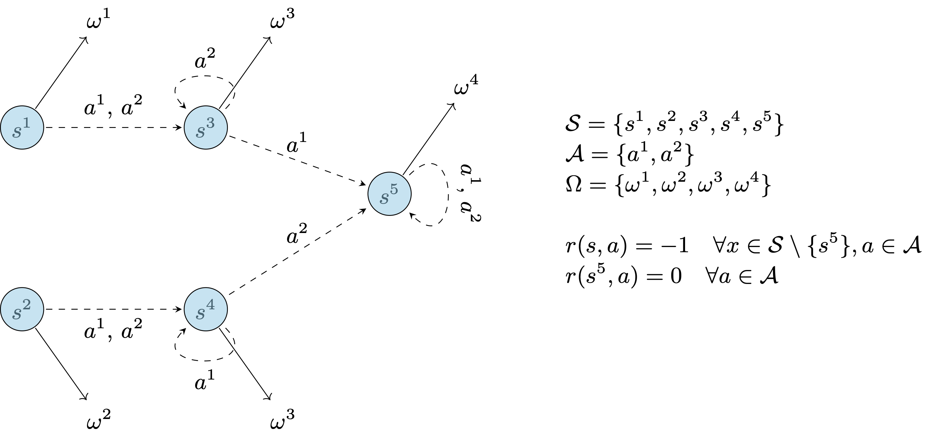
All transitions and observations are deterministic. The initial state is sampled at random in $\{s^1, s^2\}$. From the reward function, one can see that an optimal agent will reach the state $s^5$ as quickly as pocible. Any Markov policy that uses only the current observation would be suboptimal since the observation is the same in state $s^3$ and $s^4$, yet both states require different actions to reach $s^5$ with probability 1. Only be remembering the observation that was received in the previous round can a policy systematically play the optimal action (e.g., $a^1$ if the sequence of observations is ${\omega^1, \omega^3}$).

This is bad news for us. Indeed, there are many more history-dependent policy than there are stationary ones. Furthermore, in all generality, storing a history-dependant policy requires infinite memory. This is not looking good from a computational side!

Belief MDPs

The previous section bore some pretty bad news, as stationary policies are off the table if we are to preserve optimality. In this section we will see that the true story is a bit more nuanced. In particular, we’ll understand that any finite POMDPs is equivalent to a continuous, fully observed MDP – which does admit an optimal stationary policy. This MDP’s state is the so-called belief-state (or information-state): it is a sufficient summary statistic of the history, tracking the probability mass function of the POMDP’s state.

The belief-state

To introduce the belief-state, we’ll go back to the definition of the discounted reward criterion. The main idea is to realise that the objective only depends on the state distribution, conditioned on its history. Indeed, for any policy $\pi\in\Pi^\text{HR}$: $$ \begin{aligned} v_\lambda^\pi(s) &= \mathbb{E}_s^\pi\big[\sum_{t\geq1} \lambda^{t-1}r(s_t, a_t)\big]\; , \\ &= \mathbb{E}_s^\pi\big[\sum_{t=1}^\infty \lambda^{t-1} \sum_{h\in(\Omega\times\mathcal{A})^{t-1}}\sum_{s’\in\mathcal{S}} \sum_{\omega \in \Omega} r(s’, a_t)\mathbb{1}[h_{t-1}=h,\omega_t=\omega, s_t=s’] \big]\;, \\ &\overset{(i)}{=} \sum_{h\in(\Omega\times\mathcal{A})^{t-1}}\sum_{\omega\in\Omega}\left[\sum_{t\geq 1} \lambda^{t-1} \sum_{s’\in\mathcal{S}} r(s’, a_t)\mathbb{P}(s_t=s’\vert \omega_t=\omega, h_{t-1}=h)\right] \mathbb{P}_s^\pi(h_{t-1}=h, \omega_t=\omega)\;, \\ &= \mathbb{E}_s^\pi\Big[\sum_{t\geq 1}\lambda^{t-1} \sum_{s’\in\mathcal{S}} r(s’, a_t) \mathbb{P}(s_t=s’\vert \omega_t, h_{t-1})\Big] \end{aligned} $$ In $(i)$ we simply applied Bayes’ rule. We can permute every sum thanks to the dominated convergence theorem (the discounted approach is very handy in that sense).

We now see that the discounted reward directly depends on the distribution over the state, conditional to the history and the latest observation. This distribution is called the belief state:

Observe that we can now re-write the discounted cost function as: $$ v_\lambda^\pi(s) = \mathbb{E}_s^\pi\big[\sum_{t=1}^\infty \lambda^{t-1} \tilde{r}(b_t, a_t)\big] \; , $$ where we defined $ \tilde{r}(b, a) = \sum_{s\in\mathcal{S}}r(s, a)b(s)$. Note that $b_t(\cdot)$ can be represented by a vector that lives in the $\vert \mathcal{S}\vert$-dimensional simplex; we will use the notation $\pmb{b}_t$ to denote this vector.

Observability and Markovian property of beliefs

So far, nothing revolutionary: we simply re-wrote the original objective to depend directly on the belief-state. However, it turns out that the belief-state is observable (more precisely, computable) and has Markovian dynamics! Therefore, it has the same property as the state in a fully observable MDP (can you see where this is going?). Before moving on, let us explicit the claim we just made. Suppose that we have already computed $\pmb{b}_t$. (Remember that we assumed the initial distribution over was known. In other words, we have access to $\pmb{b}_0$.) After playing action $a_t=a$ and observing $\omega_{t+1}=\omega$, we have that for all $s\in\mathcal{S}$: $$ \begin{aligned} b_{t+1}(s) &= \frac{1}{\sigma(\pmb{b}_t, \omega, a)}q(\omega\vert s)\sum_{s’\in\mathcal{S}} p(s\vert s’, a)b_t(s’) \; , \end{aligned} $$ where $\sigma(\pmb{b}_t, \omega, a) = \sum_{s’’\in\mathcal{S}}q(\omega\vert s’’)\sum_{s’\in\mathcal{S}} p(s’’\vert s’, a)b_t(s’)$.

As anticipated, this identity reveals two central properties of the belief-state; (1) the belief-state is observable: provided that we know about the initial state (or the initial distribution of state) we can compute it at every round $t$ since we know $a_{t-1}$ and observe $\omega_{t}$. Further, (2) the belief-state has Markovian dynamics; as for the state in a fully observable MDP, the belief state at round $t$ only depends on the previous belief-state, the action that was input and the freshest observation.

The belief-MDP

Let’s recap: we found a summary statistic (the belief-state) which is observable and follows Markovian dynamics. Furthermore, we showed that if we defined an auxiliary reward function $\tilde{r}$, then the belief could replace the state in our objective: $$ v_\lambda^\pi(s) = \mathbb{E}_s^\pi\big[\sum_{t=1}^\infty \lambda^{t-1} \tilde{r}(\pmb{b}_t, a_t)\big] \; . $$ Packed together, those two observations have some pleasant consequences when it comes to finding optimal policies. Indeed, this establishes that solving the POMDP is equivalent to solving a fully observable MDP where the state is replaced by the belief-state. This equivalent MDP is also known as the belief-MDP. Before going any further, let us provide some details on that new MDP.

Because the belief-MDP is a fully observed MDP, the fundamental theorem of MDPs ensures that it can be solved with stationary policies. Here, stationary policies are of a particular flavor; they use a unique decision-rule $ d $ that acts directly on the belief space; $ d : \mathcal{B}=\Delta_{ \mathcal{S}} \mapsto \mathcal{A}\;. $ Once an optimal stationary policy $\tilde{\pi}^\star$ has been found in the belief-MDP, it can be exported to the original POMDP $\mathcal{M}$. At every round $t$, after having playing $a_{t-1}$ and observed $\omega_t$, we simply need to compute the belief (according to the aforementioned update rule) and apply $\tilde\pi^\star$. (Observe that for the POMDP $\mathcal{M}$, the resulting policy is actually non-stationary.)

Computational challenges

Given some POMDP, we can study its equivalent belief-MDP which has the nice property of being fully observed. This is rather pleasant, as we are left with finding stationary optimal policies for the belief-MDP. We saw in an earlier blog-post some classical control algorithms for MDPs that can do just that. However, things are, as often, slightly nuanced. Indeed, let’s not forget that the belief-state lives in $\mathcal{B}=\Delta(\mathcal{S})$ which is continuous. Algorithms like VI and PI won’t apply directly to the belief-MDP. However, it is a very natural candidate for discretisation, making it compatible with out-of-the box PI, for instance.

In all generality, finding an optimal policy in the belief-MDP is intractable because of the state space’s continuous nature. Yet, most of the control work on POMDP out there relies on it; it is just more reasonable to rely on this formulation than to blindly optimise for non-stationary policies. There are a bunch of approximation methods out there to solve belief-MDPs; you can check out the awesome monograph of [Cassandra, 1998] for a (slightly outdated?) overview on such methods.