Coming from a control background, applying RL to text generation is hardly intuitive. Is there an actual, non-degenerate dynamical system at play here? What is the concrete novelty behind the shiny LLM post-training algorithms? This post is an attempt to answer those questions by providing a semiformal derivation of the celebrated GRPO algorithm through a contextual bandit lens.

Setting

We are interested in the post-training stage of an LLM—meaning that some kind of training has already happened. More precisely, we assume access to a large transformer that has undergone pre-training (language modelling on web-scale data) and assistant finetuning (it can follow a conversational format).

The objective of post-training is loosely formulated as “getting the LLM to do something useful”. For instance, turning the LLM into a safe assistant that consistently follows some predefined rules, or getting it to solve complex tasks (e.g., mathematics, software engineering). Here, we abstract out the post-training objective through a reward function that evaluates the quality of the system’s answer to its prompt. The goal of post-training is to update the LLM so that it generates higher reward on average.

Let $\mathcal{V}\subset \mathbb{N}$ be the LLM’s vocabulary—the set of tokens it can ingest and produce. We use $c=(c_1 \ldots c_N) \in \mathcal{V}^N$ as a general notation for a prompt, and $a=(a_1 \ldots a_M) \in \mathcal{V}^M$ for an answer. LLMs generate answers “auto-regressively”; given $c$ and the answer-so-far $a_{<m} := (a_1 \ldots a_{m-1})$, an LLM $\pi$ maps $(c, a_{<m})$ to a distribution over tokens from which $a_m$ will be sampled. In other words, the probability of generating answer $a$ from prompt $c$ can be written using conditional probabilities; $$ \tag{1} \pi(a\vert c) = \prod_{m=1}^M \pi(a_m \vert c, \, a_{<m})\;. $$ The reward function $r:\mathcal{V}^N\times\mathcal{V}^M\to\mathbb{R}$ maps prompt/answer pairs to the real line. Finally, let $\mu$ be some distribution over prompts. We can now formalise the program we are trying to solve with post-training: $$ \tag{2} \max_\pi \Big\{v(\pi) := \mathbb{E}_{c\sim\mu} \mathbb{E}_{a\sim \pi(\cdot\vert c)}[r(c, a)]\Big\}\;. $$

As a dynamical system

The objective laid out in (2) does not look like one we would typically solve with reinforcement learning. To see this, recall the typical description of a dynamical system: provided a control input, some internal state updates according to some dynamics and emits an observation which can inform the next control. RL is a great tool to learn a controller in this setting, particularly when the dynamics are unknown or too complex for traditional control methods—with RL, we only need to sample from them. It provides us with routines that act as data-hungry solvers for finding near-optimal (or at least decent) controllers.

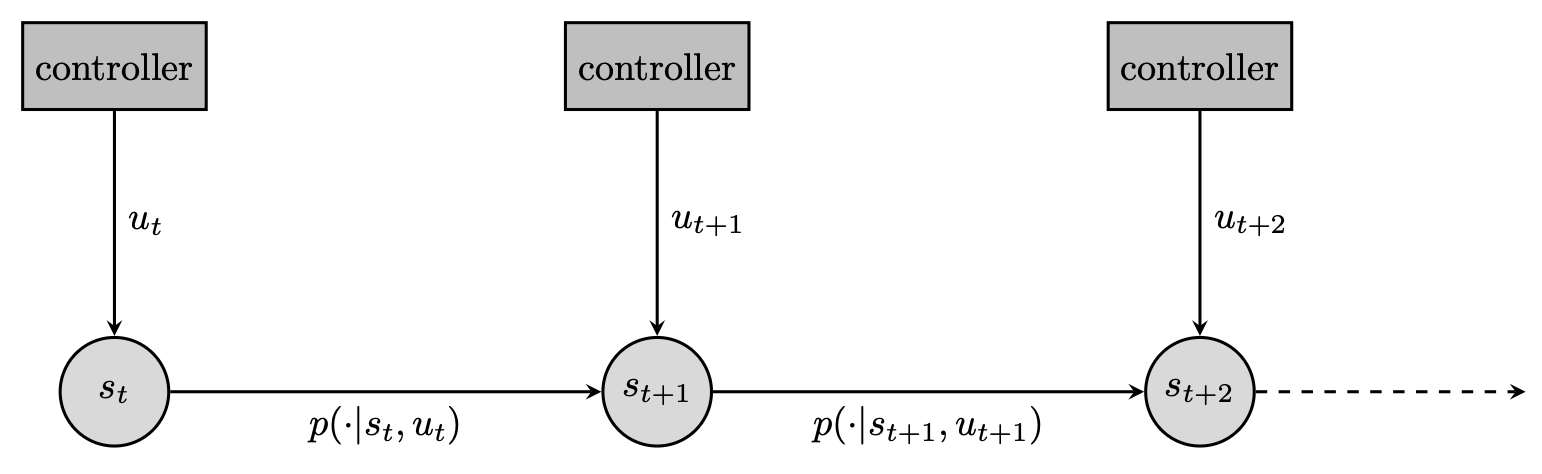
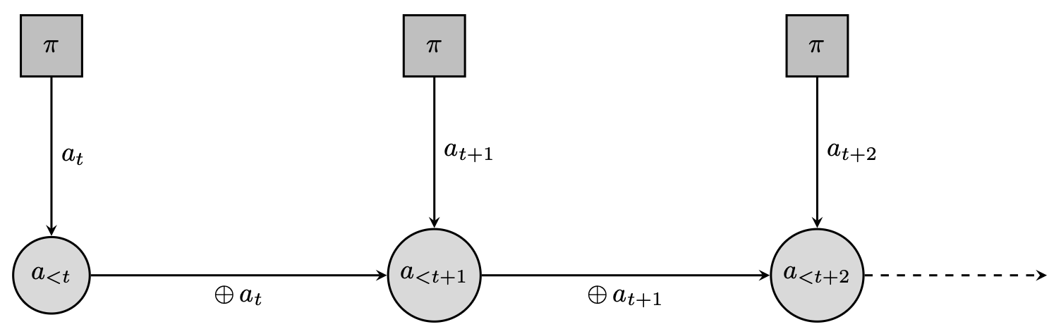
Can we formulate text-generation as a dynamical system? (We will wonder if we even should later). For instance, we could consider the emission of each token as an individual control. Concretely, the state would be the completion so far, the control a new token to append to the state, and the dynamics merely a concatenation operator. Albeit somewhat degenerate, this is a valid dynamical system. Under this formalism, we can reformulate (2) as a finite-horizon control objective; $$ \tag{3} \max_\pi \Big\{\mathbb{E}_{c\sim\mu}\sum_{m=1}^M \mathbb{E}_{a_m\sim \pi(\cdot\vert c, a_{<m})}\big[ r(c, a_{\leq m})\big] \; \text{ with } a_{\leq m} = a_{<m}\oplus a_m \text{ for all } m\leq M\Big\}\;. $$

Now, why would we want to do that? One argument is that it allows to throw the RL weaponry at post-training. You can “just apply PPO” and see where it takes you. It does feel (to me at least) quite the overkill. Earlier, we said that RL is a great tool when the dynamics are unknown or too complex; that’s not the case here, since the dynamics are just concatenation. Indeed, in (1) we were able to effortlessly write the probability of any generated trajectory (a full answer) and it did not involve any unknown quantity.

As a contextual bandit

In all fairness, folks have been applying out-of-the-box RL for post-training with quite some success. Recently it has been trendy to simplify RL algorithms for text completion. This effort is often framed as a refinement of existing algorithms; we could instead forgo the inadequate dynamical system formulation and adopt the more natural contextual bandit formalism. That’s the goal of this section. Concretely, we will re-derive the GRPO algorithm [1] from first principles and with as few tricks as possible.

Vanilla policy gradient

It is classical that one can form gradients of the objective $v(\pi)$ thanks to the log-trick: $$ \tag{4} \nabla v(\pi) = \mathbb{E}_\mu\mathbb{E}_\pi\big[r(c,a) \nabla \log\pi(a\vert c)]\;. $$

The strength of this formulation is that getting unbiased stochastic gradients boils down to sampling. We illustrate this in the following pseudocode, with a single sample. Then, post-training is essentially stochastic gradient ascent with a vanilla gradient estimator.

This protocol has two issues: variance and sample-reuse. The sample-average estimator of (4) is prone to high-variance, and the data generated to produce a gradient-estimator is thrown away after each step.

Importance sampling

Conditional generation is the bottleneck during post-training [3] ; we would like to squeeze more signal out of the data we generate and increase sample reuse. This is done via importance sampling. Consider that we are at round $t$ of our optimisation procedure; the current LLM is $\pi_t$ (recall that $\pi_0$ is the system produced by pre-training and instruction finetuning). We rewrite (4) as an expectation under $\pi_t$: $$ \tag{5} \nabla v(\pi) = \mathbb{E}_\mu\mathbb{E}_{\pi_t}\Big[\frac{\nabla\pi(a\vert c)}{\pi_t(a\vert c)} r(c,a)\Big]\;. $$

The point of (5) is that samples from $\pi_t$ can now be used for several gradient updates. We now define the next iterate $\pi_{t+1}$ as the maximiser of a surrogate off-policy objective. That is, $\pi_{t+1}\in\argmax_\pi v(\pi\|\pi_t)$ where:

$$ \tag{6} v(\pi\|\pi_t) := \mathbb{E}_\mu\mathbb{E}_{\pi_t}\Big[\frac{\pi(a\vert c)}{\pi_t(a\vert c)} r(c,a)\Big]\;. $$

One issue with importance sampling is variance, which can explode because of the importance weights. In practice, it is common to use truncated importance sampling [2] and restrict the importance weights to reasonable values. Because the maximisation of $v(\pi\|\pi_t)$ will start at $\pi=\pi_t$, we will ask for importance weights to stay close to their initial values—that is 1, for any $(c, a)$ pair. Below, we note $\vert \cdot\vert_{\ell}^{h}=\max(\ell, \min(h, \cdot))$ the clipping operator for some real-valued $\ell\leq h$. With $\varepsilon>0$, we re-define the surrogate: $$ \tag{7} v(\pi\|\pi_t) = \mathbb{E}_\mu\mathbb{E}_{\pi_t}\Big[\left\vert\frac{\pi(a\vert c)}{\pi_t(a\vert c)}\right\vert_{1-\varepsilon}^{1+\varepsilon} r(c,a)\Big]\;. $$

The following pseudocode illustrates the resulting algorithm. For simplicity, we sample a single context/answer pair per iteration. The maximiser is approximated by a few gradient ascent steps.

Control variates

To further reduce variance, we call on an old tool from statistical estimation, called control variates. We will subtract a baseline from the integrand which keeps the mean unchanged but reduces the variance of sample-average estimators. Let $b:\mathcal{V}^N\to\mathbb{R}$; then for instance: $$ \nabla v(\pi) = \mathbb{E}_\mu\mathbb{E}_\pi\big[\nabla \log\pi(a\vert c)(r(c,a) - b(c))]\;. $$ A similar result holds for the surrogate loss introduced in (6); this time the introduction of a control variate simply adds a constant term which does not change the maximiser. Below, $\blacksquare$ does not depend on $\pi$: $$ v(\pi\|\pi_t) =\mathbb{E}_\mu\mathbb{E}_{\pi_t}\Big[\frac{\pi(a\vert c)}{\pi_t(a\vert c)} \big(r(c,a)-b(c)\big)\Big] + \blacksquare\;. $$

In practice, we often/always use $b_\pi(c) := \mathbb{E}_\pi[r(c,a)]$. In this case, $A_\pi(c,a) := r(c,a) - b_\pi(c)$ is often said to represent the advantage of committing to $a$ rather than following $\pi$ on average. To properly materialise advantages, it remains to build estimators for $b_\pi(c)=\mathbb{E}_\pi[r(c,a)]$. One option is to leverage a parametric model that simply regresses the mean. Here, we will rely directly on Monte-Carlo sampling. Concretely, for every context $c$, sample $G$ answers $\{a^g\}_{g\leq G}$ from $\pi(\cdot\vert c)$ and define: $$ \hat A(c, a) := r(c, a) - \frac{1}{G}\sum_{g\leq G} r(c, a^{g})\;. $$

Putting it all together (almost) yields GRPO: at every outer round, we sample a context, generate $G$ answers under $\pi_t$, score them and estimate advantages. The inner loop maximises the clipped, advantage-weighted surrogate via gradient ascent. The sample-average estimator for the surrogate writes: $$ \tag{8} v(\pi\|\pi_t) \approx\frac{1}{G}\sum_{g\leq G} \left\vert\frac{\pi(a^g\vert c)}{\pi_t(a^g\vert c)}\right\vert_{1-\varepsilon}^{1+\varepsilon} \hat A(c, a^g)\;. $$

Finishing touches

We are almost done rederiving GRPO. We only need a few more “tricks”. The first is a classical regularisation of the post-trained system so that it does not stray too far from the pre-trained one. This is enforced by a Kullback-Leibler divergence penalty term $\mathbb{E}_\mu[\text{KL}(\pi(\cdot\vert c)\|\pi_0(\cdot\vert c))]$. Per-token estimators can be built thanks to the conditional structure of generating answers; for any $c$: $$ \tag{9} \text{KL}(\pi(\cdot\vert c)\|\pi_0(\cdot\vert c)) \approx \sum_{m=1}^M\log\frac{\pi(a_m\vert c, a_{<m})}{\pi_0(a_m\vert c, a_{<m})}\quad \text{ where } a_m\sim\pi_t(\cdot\vert c, a_{<m})\;. $$

Our last modification involves another token-level consideration. The importance weights: $$ \frac{\pi(a\vert c)}{\pi_t(a\vert c)} = \prod_{m=1}^M \frac{\pi(a_m\vert c, a_{<m})}{\pi_t(a_m\vert c, a_{<m})}\;, $$ involve a product of ratios; it’s reasonable to expect them to be ill-behaved for long answers ($M\gg 1$) given that each factor is a new potential blow-up. Clipping sure helps—yet we might end up doing it quite aggressively, which slows down learning. In practice, given that $\pi\approx \pi_t$ (cf. the regularisation towards $\pi_0$), we can obtain better-behaved object by approximating the product via a sum; with $\blacksquare$ a constant w.r.t $\pi$: $$ \prod_{m=1}^M \frac{\pi(a_m\vert c, a_{<m})}{\pi_t(a_m\vert c, a_{<m})} \approx \sum_{m=1}^M \frac{\pi(a_m\vert c, a_{<m})}{\pi_t(a_m\vert c, a_{<m})} + \blacksquare\;. $$

This motivates the following final form for the surrogate loss: $$ \tag{10} v(\pi\|\pi_t) = \frac{1}{G}\sum_{g\leq G}\hat{A}(c, a^g)\sum_{m\leq M}\Big\vert \frac{\pi(a_m\vert c, a_{<m})}{\pi_t(a_m\vert c, a_{<m})}\Big\vert_{1-\varepsilon}^{1+\varepsilon}\;. $$ Observe that clipping now happens to each importance weights individually, and not uniformly to the sum. Up to some minor algorithmic details, that’s it—we have derived GRPO not as a simplification of PPO applied to the token-level MDP, but from a bandit perspective. The following pseudocode ties it all together.

About multi-turn

For multi-turn interactions, dynamical systems become a relevant formalism again. In this setting, a trajectory is not limited to a prompt/answer pair. Many examples exist but for concreteness we focus below on reasoning. Overall, the point here is that even for multi-turn, it is rare that having a control abstraction down to the token-level makes sense.

An LLM is said to “reason” when it goes through a chain of thought before completing its answer. Reasoning is often approached as a dynamical system similar to the one described in Fig 2; the state is the answer so far. The action is however not a single token, but a variable-length utterance $\bar{a}\in\mathcal{V}^*$. The final state at termination is given by $(c, \bar{a}_1, \ldots \bar{a}_L)$. This formalism is useful if we can get external reinforcement for each utterance, evaluating its relevance towards producing a correct answer; concretely, $r(c, \bar{a}_1, \ldots \bar{a}_l) \neq 0$ for some/all $l\leq L$. In the LLM world, it is called process supervision [7] [8] and typically involves human intervention. Properly leveraging this feedback calls for an acknowledgement of the temporal dependencies—and then, the use of an actual RL algorithm.

References