Oldies but goodies: Ergodic Theorem

The goal of this blog post is to provide a self-contained proof of the so-called fundamental theorem of Markov chains. It states that provided some basic properties (spoiler: ergodicity) any Markov chain random walk converges to the same limiting distribution—irrespective of the starting state. A hidden goal is to introduce some important tools for the analysis of the average-reward criterion in MDPs.

$\quad$ In this post we abundantly mix functional and vectorial notations. Given some finite set $\mathcal{X}$, any real-valued function $f$ on $\mathcal{X}$ will be associated a vector $\mathbf{f}\in\mathbb{R}^{\vert \mathcal{X}\vert}$ where $\mathbf{f}_x = f(x)$ for $x\in\mathcal{X}$.

ⓘ

Warm-up

We will now go through some useful definitions, tools and identities we will need on our journey. First, we should once again properly state said journey’s goal, which is to prove that: $$ \textit{any ergodic Markov chain converges to its unique stationary distribution, no matter where it started.} $$ The actual meaning of this statement will hopefully become clearer and clearer through this post.

▶ Note

Notations

Let $\mathcal{X} = \{ 1, \ldots, n\}$ with $n<\infty$. We are interested in random walks $\{ X_t \}_t$ over $\mathcal{X}$ that satisfy the strong Markov property. Formally, this requires that for any $(x_1, \ldots, x_{t+1})\in\mathcal{X}^{t+1}$: $$ \begin{aligned} \mathbb{P}(X_{t+1}=x_{t+1} \vert X_{1:t} = x_{1:t}) &= \mathbb{P}(X_{t+1}=x_{t+1} \vert X_{t} = x_{t})\;, \\ &=: p_t(x_{t+1} \vert x_t) \; . \end{aligned} $$ Such a process is memory-less: future values, conditionally on the whole history, depend only on the last value. We also restrict our attention to time-homogeneous processes, such that $p_t = p$ is independent of the time $t$. The function $p: \mathcal{X} \mapsto \Delta_\mathcal{X}$ is called a transition kernel: $$ p(\cdot\vert x) = \mathbb{P}(X_{t+1}=\cdot \vert X_t=x)\;. $$ It is often represented via a matrix $\mathbf{P}\in\mathbb{R}^{n\times n}$ where given $x, y\in\mathcal{X}$, one defines $ \mathbf{P}_{xy} := p(y\vert x). $ Together with some initial distribution $\nu\in\Delta_\mathcal{X}$, it fully defines a Markov chain over $\mathcal{X}$.

$$ \mathcal{M} =(\mathcal{X}, \mathbf{P}, \nu) \; . $$

Markov chain

Overloading previous notations, we will denote $p_t(\cdot\vert x)$ the probability mass function occupied by $X_t$ conditionally on $X_0 = x$. Concretely, for $x, y\in\mathcal{X}$ we let $ p_t(y\vert x) = \mathbb{P}(X_t = y \vert X_0 =x) $. This p.m.f will be given a row vector notation $\mathbf{p}_t(\cdot\vert x)$. For instance, we will write: $$ p_t(y\vert x) = \mathbf{p}_t(\cdot\vert x) \mathbf{y}\;, $$ where $\mathbf{y}$, in this context, is a column vector one-hot representation of $y$.

Stepping the chain

A useful result regards iterating the matrix $\mathbf{P}$. In particular, for any $x\in\mathcal{X}$ one has: $$ \mathbf{p}_t(\cdot\vert x) = \mathbf{p}_{t-1}(\cdot\vert x) \mathbf{P} \; . $$ (Recall that we are using line vector – the above expression does make sense.) Iterating we obtain: $$ \tag{1} \mathbf{p}_t(\cdot\vert x) = \mathbf{x}^\top \mathbf{P}^t\; . $$ The main message is that by multiplying some distribution vector by $\mathbf{P}$ on the right, we are able to step the Markov chain by one unit of time.

▶ Proof

State classification

The states $x\in\mathcal{X}$ of a Markov chain can be classified into different categories, based on how often they are visited by a random walk. For any $x\in\mathcal{X}$ let $\tau_x$ be the stopping time measure the first return to $x$: $$ \tau_x := \min\{{t\geq 1}, \; X_t = x \text{ given } X_0 =x \} \; , $$ with the convention that $\min\emptyset = +\infty$. States such that $\mathbb{P}(\tau_x < +\infty)=1$ are called recurrent states. Others, which check $\mathbb{P}(\tau_x < +\infty)<1$ are called transient. Briefly, transient states will, at one point, stop being visited by any random walk on $\mathcal{M}$ – while recurrent states will always be visited.

▶ Note

Irreducibility

We say that some state $y$ is reachable from $x$, denoted $x\rightarrow y$ if it exists $t\in\mathbb{N}$ such that $p_t(y\vert x) > 0$. Further, $x$ and $y$ are said to communicate, denoted $x\leftrightarrow y$, if $x\rightarrow y$ and $y\rightarrow x$. A subset $\mathcal{X}^\prime\subseteq \mathcal{X}$ is said to be irreducible if all of its members communicates only with each others. All the states inside an irreducible set $\mathcal{X}^\prime$ share the same recurrence property: they are either all recurrent, or all transient.

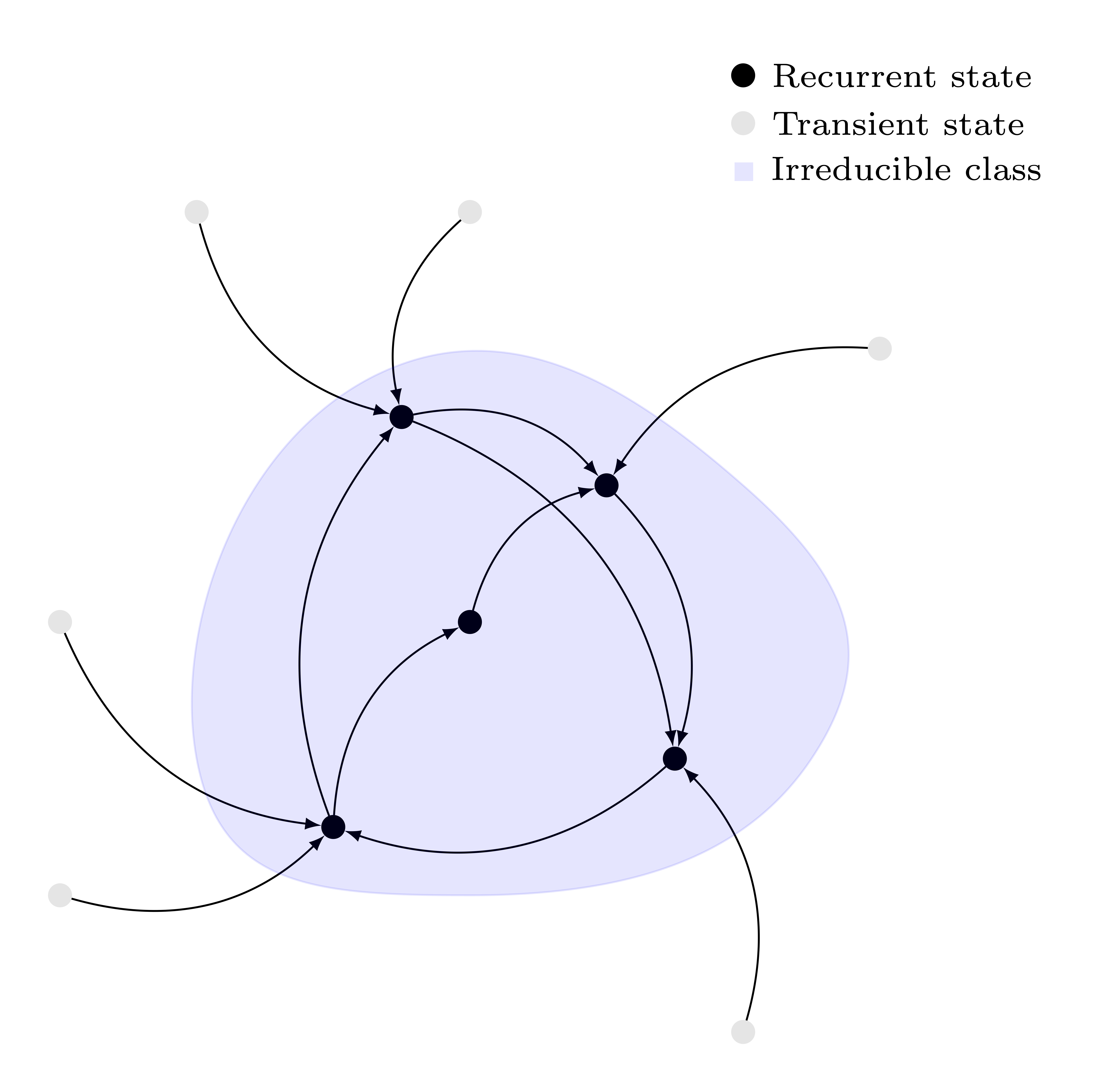
A Markov chain is irreducible if all states $x$ are recurrent and within the same irreducible class. It is straightforward to understand why irreducibility is a necessary condition for the ergodic theorem. In a Markov chain with several irreducible classes, the limiting distribution will be necessarily dependent on the starting state (it will be a function of which irreducible class the random walk was started from).

Aperiodicity

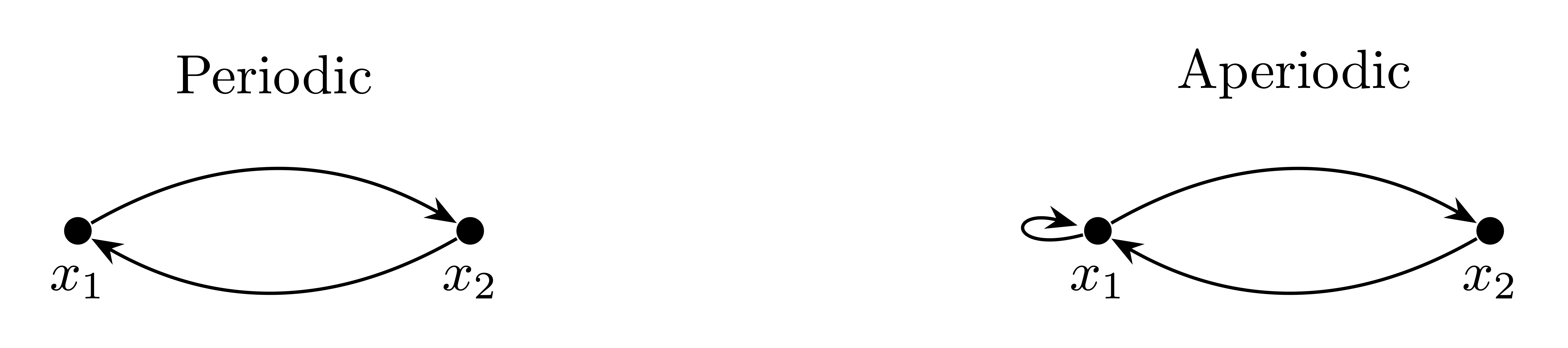
Another important state property for studying ergodicity is periodicity. The period $T_x$ of a state $x$ is defined as the greatest common denominator of the length of all paths joining $x$ to itself with positive probability: $$ T_x = \text{gcd}\{t\geq 1 \text{ s.t } p_t(x\vert x)>0\}\; . $$ It is fairly easy to show that within an irreducible class, all the states have the same periodicity. If $T$ is the period of an irreducible Markov chain, then $T=1$ leads us to call this chain aperiodic.

▶ Proof

Again, it is fairly intuitive that periodicity is a necessary requirement for something like the ergodic theorem to emerge. Below is illustrated a basic periodic Markov chain, with period $T=2$. It is clear that $p_t(\cdot\vert x_1) = (1, 0)$ for any $t\in 2\mathbb{N}$, and $p_t(\cdot\vert x_1) = (0, 1)$ otherwise. Therefore, $p_t(\cdot\vert x_1)$ does not admit a limit, and the ergodic theorem falls short.

Ergodicity

Irreducibility and aperiodicity are two necessary conditions for a result like the ergodic theorem to emerge. It turns out that together, they are also sufficient. A Markov chain checking both properties is called ergodic. An important property of ergodic chains concerns their transition matrix. If $\mathcal{M} = (\nu, \mathbf{P})$ is ergodic, then: $$ \tag{2} \exists t^\star \text{ s.t. } \mathbf{P}^t > 0 \text{ for all } t\geq t^\star\,. $$

By $\mathbf{P}^t > 0$, we mean that for all $x, y\in\mathcal{X}$ we have $[\mathbf{P}^t]_{xy}> 0$, i.e. $p_{t}(y\vert x) > 0$. This means an ergodic Markov chain starting from any point, after waiting long enough, has a positive probability of being in any state.

▶ Proof

Total-variation distance

Proving the ergodic theorem will involve showing that some notion of distance between probability distributions over $\mathcal{X}$ decreases over time. The distance we will be interested in is the total-variation distance; for any p.m.f $\mu$ and $\nu$ over $\mathcal{X}$: $$ \begin{aligned} \lVert \mu - \nu \rVert_{\tiny \text{TV}} :&= \sup_{\mathcal{Y}\subseteq \mathcal{X}} \mu(\mathcal{Y}) - \nu(\mathcal{Y})\;, \\ &= \frac{1}{2}\sum_{x\in\mathcal{X}} \vert \mu(x) - \nu(x) \vert\; .\tag{3} \end{aligned} $$

Ergodic Theorem

We will now list several equivalent formulations of the ergodic theorem. They all boil down to the same property: that the distribution followed by a Markov chain process converges to a limiting distribution, that is independant of the initial state. This is an important result; whenever we are interested in any long-term behaviour, we can safely ignore the initial conditions and focus on said limiting distribution.

$\qquad\quad\qquad\qquad\qquad\qquad\text{It exists }\pi \in \Delta(\mathcal{X})\text{ such that for any } x\in\mathcal{X}$: $$ \tag{5} \lim_{t\to\infty} \lVert p_t(\cdot \vert x) - \pi \rVert_{\text{\tiny TV}} = 0 $$

Ergodic Theorem (1/3)

The distribution $\pi$ is called a stationary distribution. The reason for this name is that any process starting under $\pi$ finds itself in the same distribution after one step of the Markov chain. One can write this as: $$ \tag{6} \boldsymbol{\pi} \mathbf{P} = \boldsymbol{\pi} \; . $$

▶ Proof

As defined in (6) the stationary distribution is a left-eigenvector of $\mathbf{P}$ with eigenvalue 1. We will see shortly that this uniquely defines $\boldsymbol{\pi}$. Using vectorial notations, we can rewrite the ergodic theorem as follows.

$\qquad\quad\qquad\qquad\qquad\qquad\text{It exists }\pi \in \Delta(\mathcal{X})\text{ such that:}$ $$ \lim_{t\to\infty} \mathbf{P}^t = \begin{pmatrix}\boldsymbol{\pi} \\\ \boldsymbol{\pi} \\\ \vdots \\\ \boldsymbol{\pi} \end{pmatrix} $$

Ergodic Theorem (2/3)

Sometimes, the ergodic theorem writes much like the law of large numbers. The next statement embodies the fact that, with Markov chains, the temporal average is the spatial average.

$\qquad\quad\qquad\qquad\qquad\qquad\text{Let $\mathcal{M}=(\mathcal{X},\mathbf{P})$ a Markov chain. Then, if } \pi \text{ is its stationary distribution, we have}\\\text{ that for any } f:\mathcal{X}\mapsto \mathbb{R}:$ $$ \lim_{t\to\infty} \frac{1}{t}\sum_{k=1}^t f(X_k) = \sum_{x\in\mathcal{X}} \pi(x)f(x) = \mathbf{E}_{X\sim\pi}[f(X)]\; . $$

Ergodic Theorem (3/3)

A proof based on coupling

Before diving in va first proof for the ergodic theorem, we need an important result. It will indeed prove convenient to establish that the stationary distribution is properly defined via $\boldsymbol{\pi} = \boldsymbol{\pi}\boldsymbol{P}$. We can then focus on the convergence of $p_t(\cdot\vert x)$, already having a properly defined candidate for the limit. To do so, we will rely on the following fundamental result: $$ \textit{Every ergodic Markov chain admits a unique stationary distribution }\pi \; . $$

▶ Note

▶ Proof

We will prove here only the existence – unicity is demonstrated using similar tools. It is enough to prove the existence of a non-zero vector $\boldsymbol{\nu}$ with positive entries such that $\boldsymbol{\nu}\mathbf{P}= \boldsymbol{\nu}$ (we will obtain our desired result up to renormalisation of $\boldsymbol{\nu}$). For some $x\in\mathcal{X}$ let $\boldsymbol{\nu}$ be the expected number of visits to each state in $\mathcal{X}$, between two consecutive visits of $x$: $$ \begin{aligned} \nu_y &:= \mathbb{E}\left[ \sum_{t\leq \tau_x} 1[X_t = y] \middle\vert X_0 = x\right]\; ,\\ &= \mathbb{E}\left[ \sum_{t\leq \infty} 1[X_t = y, t \leq \tau_x] \middle\vert X_0 = x\right]\;, \\ &= \sum_{t\leq \infty} \mathbb{P}\left(X_t=y, t\leq \tau_x \middle\vert X_0=x\right)\; . \end{aligned} $$ with $\tau_x := \min\{{t\geq 1}, \; X_t = x \text{ given } X_0 =x \}$ (we have $\tau_x <\infty$ a.s. by the chain’s irreducibility.) Observe that for any $z\in\mathcal{X}$: $$ \begin{aligned} \sum_{y} \nu_y \mathbf{P}_{yz} &= \sum_y \sum_{t\leq \infty} \mathbb{P}\left(X_t=y, t\leq \tau_x \middle\vert X_0=x\right)\mathbf{P}_{yz}\;, \\ &=\sum_{t=1}^\infty \sum_y \mathbb{P}\left(X_t=y, t\leq \tau_x \middle\vert X_0=x\right)\mathbb{P}(X_{t+1} = z \vert X_{t}=y)\;, \\ &= \sum_{t=1}^\infty \mathbb{P}\left(X_{t+1}=z, t\leq \tau_x \middle\vert X_0=x\right)\;, \\ &= \mathbb{E}\left[ \sum_{t\leq \tau_x} 1[X_{t+1} = z] \middle\vert X_0 = x\right] \;, \\ &= \mathbb{E}\left[ \sum_{t=2}^{\tau_x} 1[X_{t} = z] \middle\vert X_0 = x\right] + \mathbb{E}\left[1[X_{\tau_x + 1} = z] \middle\vert X_0 = x\right] \;, \\ &= \mathbb{E}\left[ \sum_{t=2}^{\tau_x} 1[X_{t} = z] \middle\vert X_0 = x\right] + \mathbb{E}\left[1[X_{\tau_x + 1} = z] \middle\vert X_{\tau_x} = x\right] \;, \\ & \overset{(i)}{=} \mathbb{E}\left[ \sum_{t=2}^{\tau_x} 1[X_{t} = z] \middle\vert X_0 = x\right] + \mathbb{E}\left[1[X_{1} = z] \middle\vert X_{0} = x\right] \;, \\ &= \mathbb{E}\left[ \sum_{t\leq \tau_x} 1[X_{t} = z] \middle\vert X_0 = x\right] \;, \\ &= \nu_{z}\; . \end{aligned} $$ In $\text{(i)}$, we simply used the strong Markov property. This proved the claimed result that $\boldsymbol{\nu}\mathbf{P}= \boldsymbol{\nu}$.

Reminders on coupling

We will use a line of proof that uses coupling. Given two distributions $\mu$ and $\nu$ over $\mathcal{X}$, we say that $\omega$ is a coupling of $(\mu, \nu)$ if for all $x, y\in\mathcal{X}$: $$ \begin{aligned} \sum_{y} \omega(x, y) &= \mu(x)\;, \\ \sum_{x} \omega(x, y) &= \nu(y) \;. \\ \end{aligned} $$ In other words, $\mu$ and $\nu$ are $\omega$’s marginal.

▶ Note

The fundamental result we will use is known as the coupling inequality. Let $\omega$ a coupling of $(\mu, \nu)$, and $(X, Y) \sim \omega$. Then: $$ \tag{7} \lVert \mu - \nu \rVert_{\text{TV}} \leq \mathbb{P}(X \neq Y) \; . $$

▶ Proof

The meet-and-stick coupling

We will now build a coupling that will lead us to the ergodic theorem via the coupling inequality. Consider some process $X_t$ following a random walk over our Markov chain, with some arbitrary starting point $x\in\mathcal{X}$. On the other hand, let $Y_t$ evolve according to the same random walk, yet initialised via $Y_0 \sim \pi$ – so that for any $t\geq 1$ we have that $Y_t\sim\pi$, since $\pi$ is stationary. Let $N_x$ the first time $X_t$ and $Y_t$ meet: $$ N_x := \inf\{t\geq 1, \; X_t = Y_t\}\; . $$ After this “meeting” round, we will “stick” both processes: $X_t = Y_t$ for all $t\geq N_x$. Observe that, thanks to ergodicity, both must meet after a finite time. In other words $\mathbb{P}(N_x = \infty) = 0$. (Indeed, we know that after some time $t^\star$ we have $p_{t^\star}(y\vert x)>0$ for any $y\in\mathcal{Y}$). By the coupling inequality (7) we have that: $$ \begin{aligned} \left\lVert p_t(\cdot\vert x) - \pi\right\rVert_{\text{TV}} &\leq \mathbb{P}(X_t \neq Y_t) \;, \\ &= \mathbb{P}(t\leq N_x)\; . \end{aligned} $$ Therefore, $\lim_{t\to\infty} \left\lVert p_t(\cdot\vert x) - \pi\right\rVert_{\text{TV}} = 0$, and there we have our proof!

A proof based on the Perron-Frobenius theorem

We now go through another proof that completely ignores the probabilistic rooting of Markov chains. Instead, we will use only linear algebra. (What makes the beauty of Markov chain in my eyes is the versatility of tools we can use to study them.)

The main result we will use is the Perron-Frobenius theorem. Recall that we use the following notation: for $\mathbf{A} = (a_{ij})$, $\mathbf{A}>0$ (or $\mathbf{A}$ is positive) means that $a_{ij}>0$ for all $i, j$.

$\qquad\qquad\qquad\qquad\qquad\qquad\;\; \text{Let }\mathbf{A}\in\mathbb{R}^{n\times n} \text{ be a positive square matrix, and } \text{Sp}(\mathbf{A}) \text{ its eigenvalues. Then:}\\$ $$\begin{aligned} 1.& \exists\lambda_1 \in \text{Sp}(\mathbf{A}) \text{ s.t } \lambda_1\in\mathbb{R} \text{ and } \lambda_1 \geq \vert \lambda_j\vert \text{ for all }j\neq 1\;, \\ 2.& \exists \mathbf{v} \in \mathbb{R}^n \text{ s.t. } \mathbf{A}\mathbf{v} = \lambda_1 \mathbf{v} \text{ and } \mathbf{v} >0\; . \end{aligned} $$

Perron Frobenius Theorem

Bluntly, the Perron-Frobenis identifies, for positive matrices, a real-valued leading eigenvalue $\lambda_1$ dominating all others (other eigenvalues can be complex). Its associated eigenvector can be chosen so that all of its entries are strictly positive.

At first sight, it is unclear how this helps us. The transition matrix $\mathbf{P}$ is not positive (only non-negative, $\mathbf{P}\geq 0$). For the sake of simplicity, let us cheat: we already now (see above) that $\mathbf{P}^t$ is a convergent sequence. All of its subsequences therefore converge—in particular, so does the sequence $\{(\mathbf{P}^{t^\star})^k \}_k$. It is enough to study the convergence of this last sequence, which depends only $\mathbf{P}^{t^\star}$. And, as we saw in (2), $\mathbf{P}^{t^\star}$ is positive!

$\quad$ This is an hand wavy argument that takes the problem by its solution. The point is to somewhat justify that we can assume without loss of generality that $\mathbf{P}>0$–our working assumption from now on.

⚠

It is fairly straightforward to prove that for positive stochastic matrix $\mathbf{P}$ the leading eigenvalue is $\lambda_1=1$.

▶ Proof

Since $\mathbf{P}$ and $\mathbf{P}^\top$ share the same eigenvalues, and because the Perron-Frobenius theorem also applies to $\mathbf{P}^\top$, we conclude that there is a line vector $\mathbf{v}$ with positive entries such that $\mathbf{v}\mathbf{P} = \mathbf{v}$. By rescaling $\mathbf{v}$, we obtain that there is a unique $\boldsymbol{\pi}$, with positive entries, such that $\lVert \boldsymbol{\pi}\rVert_1 = 1$ and $\boldsymbol{\pi}\mathbf{P} = \boldsymbol{\pi}$. We have just proven the existence and uniqueness of the stationary distribution!

Let’s now go one step further and prove the ergodic theorem itself. Because we are using linear algebra tools, you can already guess that we are after the formulation (2/3) of the ergodic theorem. The proof relies on the Jordan decomposition of a square matrix. Thanks to the Perron-Frobenius theorem, we know that the Jordan decomposition of $\mathbf{P}$ writes: $$ \mathbf{P} = \mathbf{Q}\begin{pmatrix} 1 & 0 & \ldots &\ldots\\ 0 & J_2 & 0 & \ldots\\0 & 0 & \ddots & 0\\ \ldots & 0 & 0 & J_n \end{pmatrix} \mathbf{Q}^{-1}, \quad \text{with } J_i = \begin{pmatrix} \lambda_i & 1 & 0 &\ldots & 0 \\ 0 & \lambda_i & 1 &\ddots & \vdots \\ \vdots & \ddots &\ddots & \ddots & 0 \\ 0 & \ddots & \ddots &\ddots & 1 \\ 0 &\ldots & \ldots & 0 & \lambda_i\end{pmatrix}\;, $$ and $\mathbf{Q}$ some non-singular matrix. From this one can show that: $$ \mathbf{P}^\infty = \lim_{n\to\infty}\mathbf{P}^n = \mathbf{Q}\begin{pmatrix} 1 & 0 & \ldots &\ldots\\ 0 & 0 & 0 & \ldots\\0 & 0 & \ddots & 0\\ 0 & 0 & 0 & 0 \end{pmatrix}\mathbf{Q}^{-1}\;, $$ by using the fact that all $J_i$ are nilpotent, since $\lambda_i<1$. In others words, $\mathbf{P}^\infty=\lim_{n\to\infty}\mathbf{P}^n$ exists and is a rank one matrix. Because $\mathbf{P}^\infty$ must be a stochastic matrix ($\mathbf{P}^n$ is stochastic for any $n\in\mathbb{N}$), we conclude that all its ranks sum to $1$. Under this constraint, the only possibility for $\mathbf{P}^\infty$ to be of rank 1 is that all of its rows are equal. We conclude that there exists a line vector $\mathbf{q}$ such that: $$ \mathbf{P}^\infty = \begin{pmatrix} \mathbf{q} \\ \vdots \\ \mathbf{q}\end{pmatrix}\;. $$

Further, one can show that this line vector checks $\mathbf{q} \mathbf{P} = \mathbf{q}$ – the stationary distribution characterisation.

▶ Proof

By unicity of the stationary distribution, we can safely conclude that $\mathbf{q} = \boldsymbol{\pi}$. We can now rest, as we just proved the formulation (2/3) of the ergodic theorem: $$ \mathbf{P}^\infty = \begin{pmatrix} \boldsymbol{\pi}\\ \vdots \\ \boldsymbol{\pi}\end{pmatrix}\; . $$

Resources

[1] is a nicely written book on Markov Chains, that goes well beyond “just” stationary distributions.

[2] is a collection of various proofs for the ergodic theorem.

[3] is a pretty neat course on Markov Chains.

If you’re interested in convergence rates and mixing times, I really enjoy this.